
4
th
ENTSO-E Guideline for Cost
Benefit Analysis of Grid Development
Projects
Version 4.1 for ACER/EC/MS opinion
24 April 2023

Foreword
This document presents the fourth version of the ENTSO-E Guideline for Cost Benefit Analysis of Grid
Development Projects (short: 4
th
CBA Guideline).
This updated guideline is the result of ‘learning by implementing’ and considering stakeholder suggestions
over a one-year development process initially based on the 3
rd
CBA Guideline. During this period, Member
States and National Regulators were consulted, following which the guideline was submitted for the official
opinion of the Agency for Cooperation of Energy Regulators (ACER) and the European Commission (EC).
The Regulation (EC) 2022/869 mandates that ENTSO-E drafts a European Cost Benefit Analysis (CBA)
guideline by 24 April 2023, which shall be further used for the assessment of the Ten-Year Network
Development portfolio.
The first official CBA Guideline drafted by ENTSO-E was approved and published by the EC on 5 February
2015, and the second official CBA Guideline drafted by ENTSO-E was approved by the EC on 27
September 2018 and published by ENTSO-E on 11 October 2018. The 3
rd
CBA Guideline was submitted
to the EC on 27 October 2022 for approval.
The first edition of the CBA Guideline was used by ENTSO-E to assess projects in the Ten-Year Network
Development Plan (TYNDP) 2014 and 2016. ENTSO-E registered the impact of the TYNDP project
assessment results on the European Commission Projects of Common Interest (EC PCI) process. This
experience demonstrated the need for a better guideline that enables a more consistent and comprehensive
assessment of pan-European transmission projects.
The 2
nd
CBA Guideline has a more general approach than its predecessor and assumes that the project
selection and definition, in addition to the scenario’s description, is within the frame of the TYNDP and,
therefore, not defined in the assessment guideline in detail. With this approach, ENTSO-E aims to develop
a CBA Guideline that can be used for one TYNDP as well as including strong principles that will stand for
a longer period. The 2
nd
CBA Guideline has been used by ENTSO-E to assess project benefits in the
TYNDP 2018. However, although improvements were included in the 2
nd
CBA Guideline, some so called
‘missing benefits’ were added to the TYNDP 2018 in addition to that which is defined in the 2
nd
CBA
Guideline. This, together with the constant efforts of ENTSO-E to improve the CBA Guideline, highlighted
the need for a 3
rd
version of the CBA Guideline.
The 3
rd
CBA Guideline contains improved methodologies for already existing indicators and an
introduction to new indicators. Among these, some new indicators stem from the lessons learnt from the
‘Missing Benefits’ process established for TYNDP 2018; however, the complexity of some of these new
indicators does not enable a Pan-European assessment. For this reason, the 3
rd
CBA Guideline includes new
‘non-mature indicators’, the nature of which is clarified in Chapter 3.4. On 7 November 2017, ENTSO-E
began to involve external stakeholders by hosting a public workshop to start the improvements which would
lead to a 3rd edition of the CBA Guideline. Subsequently, three work streams under public participation,
considering improvements on Security of Supply (SoS), Socioeconomic Welfare (SEW) and Storage
Projects, were organised from December 2017 to May 2018. The outcomes from these work streams were

considered for the drafting of the 3rd CBA Guideline which was presented at a public workshop on 18
December 2018. In 2019, ENTSO-E focused the work on the improvements on the 3rd CBA Guideline,
together with ACER and the EC. The updated draft 3rd CBA Guideline was presented to the stakeholders
during the open workshop on 8 November 2019 and released for public consultation on 9 November 2019.
The Guideline was officially submitted to ACER on 11 February 2020. On 6 May 2020 ACER delivered
their official opinion. ENTSO-E received the partial rejection of the 3
rd
CBA Guideline from the EC on 24
March 2022.
The 4
th
CBA Guideline follows the main idea and structure of the 3
rd
CBA Guideline, while including
corrections, clarifications, minor updates and some newly introduced concepts. A list of the main changes
compared to the 3
rd
CBA Guideline is given within the ‘Accompanying Documents’ submitted together
with the 4
th
CBA Guideline. Some were already included within the TYNDP 2022 Implementation
Guidelines.
Why is the 4
th
CBA Guideline important?
• It is the only European guideline that consistently allows the assessment of TYNDP
transmission and across Europe.
• The outcomes of the CBA Guideline represent the main input for the EC Project of Common
Interest and Projects of Mutual Interests lists.
• The European CBA Guideline can also be used as a source for national CBAs.

Table of Contents
1 Introduction .................................................................................................................... 14
1.1 Scope of the document .............................................................................................. 14
1.2 Overview of the document ........................................................................................ 16
1.3 CBA Implementation Guideline and other complementary documents ............................ 17
2 General approach ............................................................................................................ 20
2.1 Scenarios ................................................................................................................ 20
2.2 Study horizons ......................................................................................................... 21
2.3 Cross-border versus internal projects .......................................................................... 22
2.4 Modelling framework ............................................................................................... 22
2.4.1 Multi-sectorial market simulations ............................................................................23
2.4.2 Power market simulations .......................................................................................23
2.4.3 Power network simulations ......................................................................................24
2.4.4 Redispatch simulations ...........................................................................................24
2.4.5 Multi-case analysis .................................................................................................25
2.5 Reference network ................................................................................................... 25
2.6 Sensitivities ............................................................................................................. 28
3 Project assessment ........................................................................................................... 32
3.1 Multi-criteria and cost benefit analysis assessment ....................................................... 32
3.2 General assumptions ................................................................................................. 34
3.2.1 Clustering of investments ........................................................................................34
3.2.2 TOOT and PINT ....................................................................................................35
3.2.3 Transfer capability calculation .................................................................................38
3.2.4 Geographical scope ................................................................................................40
3.2.5 Investment value calculation ....................................................................................40
3.3 Assessment framework ............................................................................................. 42
3.4 Non-mature indicators .............................................................................................. 43
4 Concluding remarks ........................................................................................................ 44
5 Benefits, costs and residual impacts .................................................................................. 45

5.1 B1: Methodology for Socioeconomic Welfare Benefit .................................................. 52
5.2 B2: Methodology for Additional Societal benefit due to CO
2
variation ........................... 57
5.3 B3: Methodology for RES Integration Benefit ............................................................. 61
5.4 B4: Methodology for Non-Direct Greenhouse Emissions Benefit ................................... 63
5.5 B5: Methodology for Variation in Grid Losses Benefit ................................................. 66
5.6 B6: Methodology for Security of Supply: Adequacy to Meet Demand Benefit ................. 73
5.7 B7: Methodology for Security of Supply – System Flexibility Benefit ............................ 76
5.7.1 B7.1: Balancing energy exchange (aFRR, mFRR, RR) ................................................77
5.7.2 B7.2: Balancing capacity exchange/sharing (aFRR, mFRR, RR) ..................................80
5.8 B8: Methodology for Security of Supply: System Stability Benefit ................................ 81
5.8.1 B8.0: Qualitative stability indicator ..........................................................................82
5.8.2 B8.1: Frequency Stability (energy aspect) .................................................................83
5.8.3 B8.2 Frequency Stability (capacity aspect) ................................................................85
5.8.4 B8.3: Black start services ........................................................................................87
5.8.5 B8.4 Voltage/reactive power services .......................................................................87
5.9 B9: Reduction of Necessary Reserve for Redispatch Power Plants ................................. 88
5.10 C1: Methodology for CAPital EXpenditure (CAPEX) .................................................. 91
5.11 C2: Methodology for OPerating EXpenditure (OPEX) .................................................. 95
5.12 General Statements on Residual Impacts ..................................................................... 96
5.13 S1: Methodology for Residual Environmental Impact ................................................... 99
5.14 S2: Methodology for Residual Social impact ............................................................. 101
5.15 S3: Methodology for Other Residual Impact .............................................................. 103
6 Supplemental methodologies .......................................................................................... 104
6.1 Contribution to Union Energy Targets (ET) ............................................................... 104
6.2 Methodology for the assessment of Hybrid Projects ................................................... 105
6.2.1 Context ............................................................................................................... 105
6.2.2 Hybrid interconnector definition ............................................................................ 106
6.2.3 Hybrid interconnection CBA configuration ............................................................. 107
6.2.4 Radial projects: .................................................................................................... 110
6.2.5 NTCs .................................................................................................................. 110
6.3 Redispatch simulations for project assessment ........................................................... 110

6.4 Value of Lost Load ................................................................................................. 116
6.5 Climate adaptation measures ................................................................................... 117
I. Generation cost approach .............................................................................................. 119
II. Total surplus approach .................................................................................................. 120
III. Example of ΔNTC calculation ........................................................................................ 125

General definitions
Boundary
A boundary represents a barrier to power exchange in Europe. It represents a section
(transmission corridor) within the grid where the capacity to transport the power-flow
related to the (targeted level of) power exchange in Europe is insufficient.
In this context, a boundary is referred to as a section through the grid in general. A
boundary can:
• Be the border between two bidding zones or countries;
• Span multiple borders between multiple bidding zones or countries; or
• Be located inside a bidding zone or country, dividing the area into two or multiple
sub-areas.
Competing
transmission
projects/investments
Two or more transmission projects are regarded as competing if they serve the same
purpose.
In cases where competing projects are proposed to achieve a transmission capacity
increase, the projects typically (but not exclusively):
a) Increase NTC on the same boundary; and
b) Their socioeconomic viability is reduced if assessed under the assumption that the
other project is also realised. Therefore, the overall net benefit of realising both
projects is lower than the sum of the individual net benefits.
Current grid
(starting grid)
The current grid is the existing transmission grid and is determined at a specific date that
is dependent on the point in time of the respective study. It can also be considered the
starting point or initial state of building the reference grid by including the most probable
projects as described in this 4
th
CBA Guideline.
Generation power
shift
Generation power-shift is the deviation from the cost-optimal power plant dispatch
(determined by market simulations) for the purpose of influencing grid utilisation.
1
It
considers the loading of a line across a boundary that separates system A from system B
(with energy transported from A to B), arrived at as a result of optimum dispatch.
Generation is incrementally increased in area A and decreased in area B. This process is
conducted up to the point where the line loading security criteria in System A or System
B are reached. The volume of the power shift represents the additional market exchange
possible between these systems and should be reflected by the variation in NTC that is
assumed in market simulations. Generation power shift is used to modify the market
exchange across a specified boundary to find the maximum change in generation made
possible by the grid.
Grid Transfer
Capacity (GTC)
The GTC is defined as the greatest (physical) power-flow that can be transported across
a boundary without the occurrence of grid congestions, considering standard system
security criteria.
1
This can also be seen as the definition of the re-dispatch. To avoid confusion in this case it is referred to generation power-shift as in reality the
re-dispatch is used to reduce the grid utilisation and to heal congestions. However, as described in this guideline, the re-dispatch will also be used
to determine the theoretical maximum grid utilisation by bringing the system to the edge of security.

Hybrid Projects
A hybrid project is a project which enables an interconnector function between bidding
zones (either onshore or offshore) while simultaneously facilitating a client connection
with a certain technology (RES or non-RES; generation or load; AC or DC)
Interdependent
Projects
An interdependent project is a project the realisation of which is dependent on the
realisation of another project, e.g. where a project needs to be built as a prerequisite
before the interdependent project can fulfil its full potential. This might also apply to two
or more projects interdependent from each other.
Interlinked Model
Interlinked (sector) models simulate energy market transactions and interactions with
other sectors of different energy carriers. The interlinked model is necessary to assess
projects from a ‘one energy system’ perspective.
Investment
An investment is the smallest set of assets that together can be used to transmit electrical
power and that effectively add transmission infrastructure capacity. An example of an
investment is a new circuit, the necessary terminal equipment and any associated
transformers.
Investment need
The need to develop capacity across a boundary is referred to as an investment need. As
different scenarios may result in different power flows, the amount of capacity required
to transport these power flows across a boundary and, consequently, the amount of
investment needed, is likely to differ from scenario to scenario.
Investment status
The investment status is defined depending on its stage of development, according to one
of the following six options:
• Under consideration: Investments in the phase of planning studies and under
consideration for inclusion in national plan(s) and Regional/EU-wide Ten-Year
Network Development Plans (TYNDPs) of ENTSO-E.
• Planned, but not yet in permitting: Investments included in the national
development plan and that have completed the initial studies phase (e.g. completed
pre-feasibility or feasibility study), but have not yet initiated the permitting
application.
• Permitting: Investments for which the project promoters have applied for the first
permit required for its implementation and the application is valid.
• Under construction: The investment is in its construction phase.
• Commissioned: Investments that have come into first operation.
• Cancelled.
Main investment
In the case of a project that consists of a number of investments, one investment (e.g. an
interconnector) is to be defined as a main investment with one or more supporting
investments attached. This is required when clustering investments. The main investment
is planned to achieve the specific goal, e.g. an interconnector between two bidding areas,
with the supporting investments (as part of the project) required to achieve the full
potential of that main investment. The full potential of the main investment represents its
maximum transmission capacity in normal operation conditions.

Net Transfer
Capacity (NTC)
The NTC is the maximum foreseen magnitudes of power exchange programmes that can
be operated between two bidding zones while respecting the system security
requirements of the areas involved. The NTC is used in market modelling to represent
the power exchange capability between bidding zones.
Planning cases
The representation of how the power system (i.e. the generation and transmission system)
could be managed at a point in time. They are used to represent a detailed model of the
grid for that point in time, or a snapshot, and are used in network studies. Planning cases
are selected inter alia based on:
a) The outputs from market studies, such as system dispatch, frequency and magnitude
of constraints;
b) Regional considerations, such as wind and solar profiles or cold/heat spells; and
c) Results of pan-European Power Transfer Distribution Factor (PTDF) analysis, when
available.
Project
A project is defined as a single investment or group of investments. Therefore, it can
comprise a main investment with supporting investments that must be realised together
to enable the main investment to realise its intended goal, i.e. the full potential, which is
defined as the capacity increase of the main investment. In cases where there are no
supporting investments, the project consists of the main investment alone and will
nonetheless be described as a ‘project’ in this CBA Guideline.
Put IN one at the
Time (PINT)
A methodology that considers each new investment/project (line, substation, phase
shifting transformer (PST), or other transmission network device) on the given network
structure one-by-one and evaluates the load flows over the lines with and without the
examined network investment/project reinforcement.
Radial Projects
A radial project enables the connection of a certain technology (RES or non-RES
generation) to a bidding zone.
Reference network
The reference network is the version of the network used to calculate the incremental
contribution of the project that is assessed. Therefore, it is used as the starting point for
the computation of and the respective benefit indicators.
Renewable Energy
Sources (RES)
RES means energy from renewable non-fossil sources, namely wind, solar (solar thermal
and solar photovoltaic) and geothermal energy, ambient energy, tide, wave and other
ocean energy, hydropower, biomass, landfill gas, sewage treatment plant gas, and biogas
ESAB. A detailed overview is also provided within the study specific Implementation
Guidelines.
Respective study
The study in which the CBA assessment is performed, e.g. the TYNDP.
Scenario
A set of assumptions for modelling purposes related to a possible future situation in which
certain conditions regarding demand, installed generation capacity, infrastructures, fuel
prices and global context occur.
Societal cost of CO
2
The societal cost of carbon can represent two concepts:
• The social cost that represents the total net damage of an extra metric ton of CO
2
emissions due to the associated climate change;
2
and
2
IPCC Special report on the impacts of global warming of 1.5°C (2018) - Chapter 2

• The shadow price that is determined by the climate goal under consideration. It can
be interpreted as the willingness to pay for imposing the goal as a political
constraint.
3
Take Out One at the
Time (TOOT)
A methodology that consists of excluding projects from the forecasted network structure
on a one-by-one basis to compare the system performance with and without the project
under assessment.
Ten-Year Network
Development Plan
(TYNDP)
The European Union-wide report examining the development requirements for the next
ten years, carried out by ENTSO-E every other year as part of its regulatory obligations
defined under Article 8, paragraph 10 of the Regulation (EU) 2019/943.
Time step
Simulation models compute their results at a given temporal level of detail. This temporal
level of detail is referred to as the time step. Smaller time steps generally increase
simulation run time, whereas larger time steps decrease simulation run time. Typically,
simulations are done using hourly time steps, but this level of granularity may vary
depending on the level of detail required in the results.
Abbreviations
The following list shows abbreviations used in the 4th ENTSO-E Guideline for Cost Benefit Analysis of
Grid Development Projects:
ΔNTC
Increase in NTC
AC
Alternating Current
ACER
European Union Agency for the Co-operation of Energy Regulators
aFRR
Automatic Frequency Restoration Reserve
BCR
Benefit-to-Cost Ratio
CAPEX
Capital Expenditure Cost
CBA
Cost-Benefit Analysis
CBCA
Cross-Border Cost Allocation
CE
Continental Europe
CEER
Council of European Energy Regulators
CF
Complexity Factor
CIGRE
Council on Large Electric Systems
3
IPCC Special report on the impacts of global warming of 1.5°C (2018) - Chapter 2

CONE
Cost of New Entrant
DA
Day-ahead Market
DC
Direct Current
DSR
Demand Side Response
EC
European Commission
EBGL
Electricity Balancing Guideline
EED
Energy Efficiency Directive
EENS
Expected Energy Not Served
ENTSO-E
European Network of Transmission System Operators for Electricity
ENS
Energy Not Served
EPRI
Electric Power Research Institute
ET
Energy Targets
ETS
Emissions Trading Scheme
EU
European Union
FCR
Frequency Containment Reserve
FE
Frequency Exchange
FO
Frequency Optimisation
FN
Frequency Netting
FRR
Frequency Restoration Reserve
FV
Future Value (Cost or Benefit)
GTC
Grid Transfer Capability
HVDC
High Voltage DC
ID
Intraday Market
ILM
Interlinked Model
IPS
Integrated Power System

LFC
Load Frequency Control
LOLE
Loss of Load Expectation
MES
Multi-Energy System
mFRR
Manual Frequency Restoration Reserve
MS
Member States
MSC
Mechanically Switched Capacitors
MSR
Mechanically Switched Reactors
NECP
National Energy and Climate Plan
NPV
Net Present Value
NRA
National Regulatory Authority
NTC
Net Transfer Capacity
OBZ
Offshore Bidding Zone
OHL
Overhead Line
OPEX
Operating Expenditure Cost
P2G
Power-to-Gas
PCI
Projects of Common Interest
PINT
Put IN one at the Time
PMI
Project of Mutual Interest
PP
Project Promoter
PST
Phase Shifting Transformer
PTDF
Power Transfer Distribution Factor
PV
Present Value
RES
Renewable Energy Sources
RoCoF
Rate of Change of Frequency
RR
Replacement Reserves

SA
Synchronous Area
SA-OA
Synchronous Area Operational Agreements
SEA
Strategic Environmental Assessment
SEW
Socioeconomic Welfare
SMC
Submarine Cable
SOC
System Operations Committee
SOGL
Commission Regulation (EU) 2017/1485: Establishing a Guideline on Electricity Transmission
System Operation
SoS
Security of Supply
STATCOM
Static Synchronous Compensator
SVC
Static Var Compensator
TOOT
Take Out One at the Time
TRM
Transmission Reliability Margin
TSO
Transmission System Operator
TTC
Total Transfer Capacity
TYNDP
Ten-Year Network Development Plan
UGC
Underground Cable
VOLL
Value of Lost Load
XB
Cross-border

1 Introduction
This Guideline for Cost Benefit Analysis of Grid Development Projects was prepared by the European
Network of Transmission System Operators for Electricity (ENTSO-E) in compliance with the
requirements of the EU Regulation (EU) 2022/869 on guidelines for trans-European energy infrastructure
(referred to as 'the Regulation').
This Guideline is the fourth version of this document produced by ENTSO-E (referred to as the 4
th
CBA
Guideline) and will be further updated and improved following the results of an extensive consultation
process. The consultation process plans to involve the public, stakeholder organisations, national authorities
and their national regulatory authorities, the Agency for Cooperation of Energy Regulators (ACER), and
the European Commission (EC), following the requirements as defined in the Regulation (Article 11 2.).
This updated version of the guideline (version 4.1) will be sent to Member States (MS), the EC and ACER
by 24 April 2023 following the Regulation (Article 11 1.). After receiving the feedback from theses
stakeholders, ENTSO-E will include amendments accordingly and submit the updated guideline (version
4.2) to the EC for approval.
The indicators that have been developed enable a harmonised, system-wide cost–benefit analysis (CBA) of
projects. They facilitate a uniform approach in which all projects and promoters (either TSO or third party)
are treated and assessed in the same manner.
The guideline’s primary use is to describe the projects contained in the ENTSO-E Ten-Year Network
Development Plan (TYNDP), including the Projects of Common Interest (PCI) and Projects of Mutual
Interest (PMI) that are identified from the list of TYNDP projects. It is also recommended to be used for
the cross-border cost allocation (CBCA) process as required by the Regulation (Article 16 4.(a)).
4
The methodologies developed in this Guideline are of general relevance to the electricity industry and may
therefore be useful to anyone seeking to assess transmission investments. Some of the indicators are
developed to meet specific requirements of the Regulation concerning market integration, security of supply
(SoS) and sustainability, including the integration of renewable energy and energy storage among others.
Of particular reference, the indicators are designed to comply with Article 4.3(a), Article 11, Annex IV and
Annex V of the Regulation.
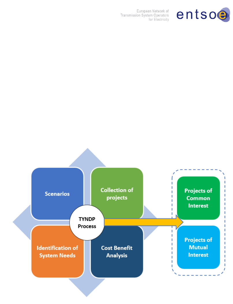
1.1 Scope of the document
The TYNDP process consists of four main processes, illustrated in Figure 1 below: the building of
scenarios, the project collection, the identification of system needs, and the CBA. This complies with the
Regulation, which requires projects to be assessed under different planning scenarios, each of which
represents a possible future development of the energy system. Although project costs are scenario
independent, the benefits strongly correlate with scenario-specific assumptions. Therefore, scenarios that
4
Additional information can be found at the ENTSO-E’s TYNDP webpage: https://tyndp.entsoe.eu/
define potential future developments of the energy system are used to gain insight into the future benefits
of transmission projects.
A system-needs assessment determines the impact of those scenarios on the transmission system,
identifying network bottlenecks and additional investment needs. This requires network power-flow,
stability and market analyses.
This document aims to provide guidance for how to perform the last step: an energy system-wide CBA.
Only where needed for the understanding of this CBA Guideline is general information on the other steps
given, whereas more detailed information and guidance about the other processes can be found on ENTSO-
E’s website.
Figure 1: Overview of the assessment process inside the TYNDP and for identifying PCIs and PMIs
The aim of the 4
th
CBA Guideline is to deliver general guidance on how to assess projects from a CBA
perspective. The Guideline describes the ENTSO-E’s criteria for performing CBA in addition to the
common principles and methodologies used in the necessary network studies, market analyses and
interlinked modelling methodologies. Because of this general approach which allows for the application to
different studies, not all study-specific details and requirements can be described in detail within the scope
of this document. In addition to the 4
th
CBA Guideline, study-specific complementary Implementation
Guidelines require publishing along with the respective TYNDP study, containing all relevant input data,
data sources and assumptions utilised in the CBA implementation. An overview of the required
complementary information, provided within the implementation guidelines and other documentation

within the TYNDP, is given in Section 1.3. The implementation guidelines for the respective TNYDP will
be part of the TYNDP package and will therefore also be publicly consulted on.
To ensure a full assessment of all transmission benefits, ENTSO-E applies a multi-criteria approach to
describe the indicators associated with each project. This means that some of the indicators are monetised,
whereas others are quantified in their typical physical units (i.e. tons or GWh). The set of common indicators
contained in this guideline form a complete and solid basis for project assessment across Europe, both
within the scope of the TYNDP as well as for project portfolio development in the PCI selection process.
5
As the TYNDP is a continuously evolving process, this document will be reviewed periodically, in line
with prudent planning practice and further editions of the TYNDP, or upon request (as foreseen by Article
11.13 of the Regulation).
1.2 Overview of the document
This CBA Guideline uses a modular approach to enable more efficient updates of the Guideline and to
allow stakeholders to better focus on specific content without necessarily going through the whole
document.
To enable the modular approach, the 4
th
CBA Guideline is structured into six main chapters, supported by
a number of detailed sections. Chapter 5 presents the indicator-specific information and provides a full
description of all the indicators. It describes the methodology to be used and defines the principles and the
requirements to properly assess the relevant indicator. Chapter 6 contains additional methodologies used in
the CBA assessment but is not indicator-specific. The application for the TYNDP is further supported with
supplemental implementation guidelines that will be provided separately.
Chapter 1 introduces the Guideline and provides a context to the indicators that have been developed for
use in CBA..
Chapter 2 discusses general approach matters. This includes, among others, a discussion regarding
scenarios and study horizons, cross-border and internal projects, reference network descriptions, and
sensitivities.
A detailed description of the overall assessment, including the modelling assumptions and indicator
structure, is given in Chapter 3. A general overview of the indicators is given in Section 3.3. This set of
common indicators forms a complete and solid basis for project assessment across Europe, both within the
scope of the TYNDP and for project portfolio development in the PCI selection process.
5
Chapter 4 concludes and provides a summary of the aim of the 4
th
CBA Guideline.
5
It should be noted that the TYNDP does not select PCI projects. Regulation (EU) 2022/869 (art 4.5) states that ‘each Group shall determine its
assessment method on the basis of the aggregated contribution to the criteria […] this assessment shall lead to a ranking of projects for internal
use of the Group. Neither the regional list nor the Union list shall contain any ranking, nor shall the ranking be used for any subsequent purpose.’

The benefit indicators, costs description and residual impacts are described in detail in Chapter 5. In Chapter
6, the details of the main concepts of the methodologies that are not indicator-specific are explained.
1.3 CBA Implementation Guideline and other complementary
documents
As the CBA Guideline is a general guidance document for the assessment of projects, it would be
impractical to include detailed methodologies, parameters or specific assumptions for the calculation of
each indicator were in this document. Therefore, the CBA Guideline needs to be complemented by
additional detailed information on how the simulations are to be performed. This additional information
requires publishing within the respective TYNDP study and shall specify which method is to be used in
the event the CBA Guideline allows for more than one possibility, as well as how to interpret the rules
defined in the CBA Guideline.
For the CBA phase of the TYNDP process, Implementation Guidelines will be prepared that contain all of
the necessary details required to calculate the indicators, considering the modelling possibilities and
assumptions that can be applied in the relevant TYNDP. Together with the Scenario Report (where all the
scenario-specific details not defined in the 4
th
CBA Guideline are given) and the Implementation Guideline,
the CBA Guideline provides an exhaustive guidance on how to perform the project specific assessment
within the TYNDP process. The Implementation Guidelines is considered a part of the TYNDP package,
and will therefore be publicly consulted on, together with the rest of the package, every other year.
Table 1 contains a summary of details for certain indicators to be defined in complementary documents,
which focus on the TYNDP process. If applied to other studies, these details must also be given within the
respective study.

Table 1: Summary of indicators for which complementary documents are to be defined.
Defined in:
Indicator or rule
Information required to be provided
Implementation Guidelines
Transfer capability calculation
Power shift method to be applied (generation shift and/or load shift; how to scale the generation units or loads in the system when
applying the power shift).
Selection of contingencies and critical branches.
Details of internal GTC calculation.
Impacts of third-countries
Method to remove the effects of non-European countries from the pan-European results and overview of the general perimeter used for
the simulations and CBA evaluation.
Assessment of commissioning years
Detailed explanation of the methodology and definition of needed parameters; the outcome of this assessment has to be given in the
project sheets
Market simulations
Value of hurdle cost to be used.
Number of climate years to be used.
Sectors to be included in the simulations
Network simulations
Mapping the market results to the network model (nodal level)
Load-flow method to be applied with explanation (whether AC or DC)
Sensitivities
The applied sensitivities together with an overview of the assessment framework that are being applied (e.g. climate years, scenarios
etc.)
List of projects to which the respective sensitivities are being applied
Motivation with explanation on the choice of the respective sensitivities
Transfer Capability Calculations
Steps of the NTC calculations process including for each step: input, modelling tools and output
For each project: the information whether power shift or load shift has been used.
For each project: the tool used for the calculation
For each project: information on whether year-round calculations or PiT have been used
Information on the usage of TRM and TTC
Percentile value used as a threshold
Geographical scope
An overview of the geographical scope on which the costs and benefits are applied needs to be given, e.g. how costs and benefits in
non-EU MS are being considered and in- or excluded from the final results.
B1. Socioeconomic Welfare
Method for reporting the part of SEW from fuel savings due to the integration of RES (SEW–RES) and the avoided CO
2
cost (SEW–
CO
2
).
In the event of redispatch simulations, a detailed description of the methodology used
For each project: the methodology used to assess each project
B2. CO
2
Emissions
Societal cost to be used.
B3. RES Integration
How to report avoided RES spillage (dump energy) from the market simulation results.

B4. Non-direct greenhouse Emission
List of emission types and factors per generation category.
Implementation Guidelines
B5. Variation in Grid Losses
Monetisation of losses on HVDCs between different market nodes.
Assumption to apply for the compensation of partial double counting with SEW.
Number of climate years to be used.
Information regarding whether points in time were used and the specific points in time used.
B6. SoS: Adequacy to Meet Demand
Method for introducing peaking units in TOOT cases.
Definition of which sanity check method is to be used.
Details of the treatment of strategic reserves
Details of Monte-Carlo approach.
Value of VOLL and CONE.
B7.1 SoS – System Flexibility Benefit
Description of the methodology of how the qualitative indicators are defined
B8.1
Detailed motivations and a clear descriptions of the chosen system splits, together with the formula and all relevant parameters for the
RoCoF calculation
B8.2. Black start services
6
Definition of the necessary assumptions
Project Costs
Definition of the costs delivered within the project sheets.
CAPEX
Table of standard costs
OPEX
Definition of a yearly percentage of CAPEX for non-mature investments
Investment value calculation
The assessment period and real discount rate could be confirmed or updated with respect to what is indicated in the CBA Guideline
Sanity check for hybrid and radial
projects assessment
Detailed methodology on how to apply the sanity check
Definition of what RES includes
To be applied for the calculation of B3 and the RES penetration ET3
Project Sheets
The content of the project sheet should be defined in the Implementation Guidelines
Storage
Information on how storage projects are modelled
Documentation
of the
respective
study
Simulation tools used to perform the
assessment
List of tools used for Market, Network and Redispatch simulations.
For each project: tool(s) used to perform the calculation
Transfer Capability Calculations
Links to the databases used in the calculations
Database
Description of the main databases used for the CBA assessment
Reference
network
Specific document on the reference grid
and Implementation Guidelines
Definition of the reference grid together with a justification for the chosen reference grid/s.
List of all projects within the reference grid
Treatment of interdependent projects
6
Or given by the project promoters

20
2 General approach
The general approach used to assess projects considers the following:
• The range of future energy scenarios and study horizons;
• Internal and cross-border considerations;
• The modelling framework to be used in undertaking the analysis;
• The identification of a reference network used to assess the impact of the reinforcement against;
• The use of multi-case analysis to simplify analysis; and
• The approach to sensitivity studies.
These are discussed in detail below.
2.1 Scenarios
Regulation (EU) 2022/869 states that ENTSO-E is required to use scenarios as the basis for the TYNDP
and for the calculation of the CBA used to determine EU funding for electricity and gas infrastructure PCI
and PMI. Consequently, ENTSO-E, together with ENTSOG, design scenarios specifically for this purpose
every two years.
The scenarios are a description of plausible futures that can be characterised by: a generation portfolio; a
demand forecast and power exchange patterns between the study region and other power systems. They
provide the framework which the future is likely to occur within, but do not attach a probability of
occurrence to them. The scenarios represent a means of addressing future uncertainties and the interactions
between those uncertainties. Some TYNDP scenarios have a stronger national focus than others; some are
‘top-down’ whereas others are ‘bottom-up’. There is no right or wrong, likely or unlikely option; all
scenarios have to be treated equally and, because of the uncertainties of the future energy sector, no scenario
can be defined as a ‘leading scenario’.
The objective of using scenario analysis is to construct sufficiently contrasting future developments that
differ enough from each other to capture a plausible range of possible futures that result in different
challenges for the grid. These different future developments can be used as input parameter sets for
subsequent simulations.
The scenarios are constructed at the level of the European electricity system and can be adapted in more
detail at a regional level. When constructed, the scenarios must reflect both European and national
legislation that is in force at the time of the analysis and its effect on the development of these elements.
The scenarios are, when possible, derived from official EU and Member-State data sources and are intended
to provide a quantitative basis for the infrastructure investment planning.
One of the key principles of the EU energy policy is the Energy Efficiency First principle. By considering
this principle in the scenarios, it is ensured that it will also be considered in products that build upon the
scenarios. The scenarios are constructed so that they align with the energy efficiency targets as they are
defined in the Energy Efficiency Directive (EU) 2018/2002 (EED). This can, for example, be observed in
21
the level of energy demand. The scenarios aim to be in line with the final energy levels as defined in the
EED or based on the latest figures available when the scenario project freezes the data.
As mentioned above, scenarios can be built as ‘bottom-up’, which means that the scenario is built based on
the National Energy and Climate Plans (NECP) from MS. According to the (EU) regulation 2018/1999,
MS are required to establish a ten-year integrated NECP for 2021–2030, outlining how it intends to
contribute, inter alia, to the 2030 target for energy efficiency. The EED states that MS should consider the
Energy Efficiency First principle for all sectors and technologies defined and should be a part of the NECP.
Consequently, the Energy Efficiency First principle is implemented via a bottom-up approach.
For the top-down scenarios, the Energy Efficiency First principle is applied on the final energy levels
according to the current regulations and these are applied by selecting the most efficient technology and
energy carrier according to the storyline. Moreover, by implementing flexibility options such as DSR, V2G,
storages and batteries within the scenario models, the energy reduction will be further helped.
Detailed information on the joint ENTSOG and ENTSO-E scenarios can be found in the respective scenario
reports.
7
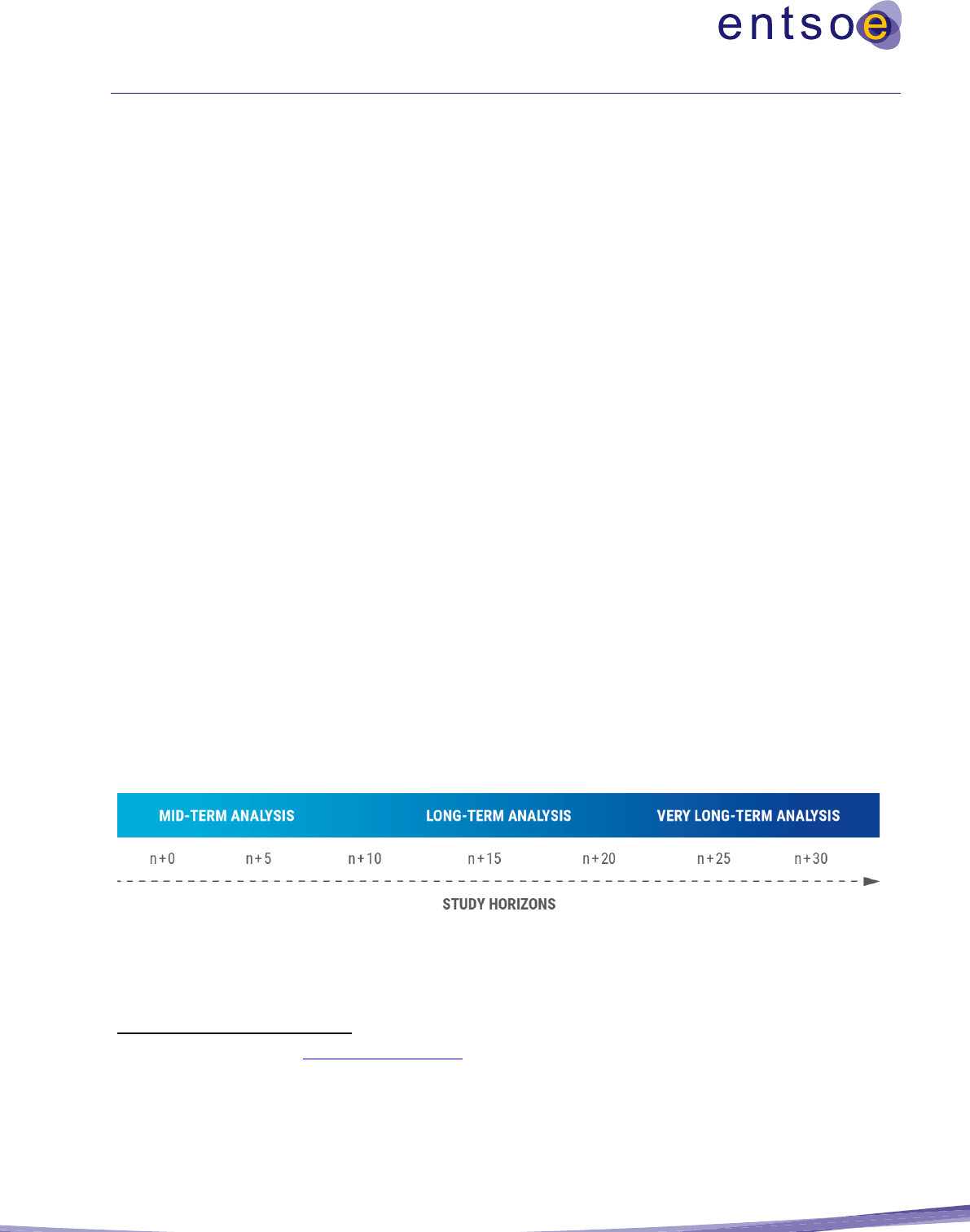
2.2 Study horizons
Scenarios can be distinguished depending on the time horizon, as illustrated in
Figure 2, and can be described as follows:
• Mid-term horizon (typically 5 to 10 years): mid-term analyses should be based on a forecast for
this time horizon;
• Long-term horizon (typically 10 to 20 years): long-term analyses will be systematically assessed
and should be based on common ENTSO-E scenarios.
• Very long-term horizon (typically 30 to 40 years). Analysis or qualitative considerations could be
based on the ENTSO-E 2050-reports; and
• Horizons which are not covered by separate data sets will be described through interpolation or
extrapolation techniques.
Figure 2: Continuous timeline with future study years and corresponding study horizons
8
.
As shown in
7
Link to the latest scenario report: TYNDP 2022 Scenario Report
8
There is no strict definition of the beginning and end of the horizons, and an overlap might appear, indicated by the gradual colour gradients
used in the figure.

22
Figure 2, the scenarios developed for the long-term perspective may be used as a bridge between the mid-
term horizon and the very long-term horizon (i.e. n+20 to n+40). The aim of the perspectives beyond n+20
should be that the pathway realised in the future should fall within the range described by the scenarios
with a reasonable level of likelihood.
The scenarios on which to conduct the assessment of the projects will be given for fixed years and rounded
to full five years (e.g. 2025 instead of 2023 for n+5 in TYNDP 2018). For the mid-term horizon, the
scenarios must be representative of at least two study years. For example, for the TYNDP 2020, the study
years of the mid-term horizon are 2025 (n+5) and 2030 (n+10).
2.3 Cross-border versus internal projects
Assessing projects using only the impact on the transfer capacities across certain international borders can
lead to an underestimation of the project-specific benefits as most projects also show significant positive
benefits that cannot be covered by only increasing the capacities of a certain border. This effect is the
strongest for, but not limited to, internal projects.
Internal projects do not necessarily have a significant impact on cross-border capacities, which makes it
difficult to assess them using market simulations that consider only one node per country without a flow-
based model.
Both internal and cross-border projects can be classified as having pan-European relevance. However, they
all develop grid transfer capability (GTC) over a certain boundary, which may, or may not, be an
international border (and sometimes several boundaries).
Depending on the types of project, a suitable method should be used. At this point, it is recognised that
there is no unified method available that can address the specific aspects of all these projects adequately.
Therefore, three alternative methods are given for the calculation of the benefits:
• Market simulations;
• Network simulations; and
• Combined market and network simulations, i.e. redispatch simulations
Both market and network simulations provide different types of information; they generally complement
one another so they are frequently used in an iterative manner. These methods are discussed in detail in the
following chapter.
2.4 Modelling framework
As the indicators described in Chapter 5 generally rely on different principles, they also need to be achieved
under the use of different models. An overview of these models, i.e. Market simulations, Network
simulations and Redispatch simulations, is given in this section.
It should be noted that most of the indicators can be achieved using more than one of the described models;
this information will be given in an overview table at the end of the respective indicator.

23
2.4.1 Multi-sectorial market simulations
In general, energy markets can be organised by exchanges. These entities collect, for a certain commodity,
buy and sell orders from consumers and producers. The orders are stacked in the form of demand and supply
curves. Under uniform price auction schemes, the markets are cleared by matching demand and supply
curves to obtain market clearing prices for the corresponding commodities. Market models are able to
capture these principles and are essential for the project assessment. By running market simulations, they
are applied to reflect realistic market outcomes.
Interlinked (sector) models or integrated multi-energy system (MES) models capture energy market
transactions and interactions with different sectors. In this regard, sectors correspond to energy carriers for
which corresponding markets for energy trading exist. MES models could contain energy carriers such as
electricity, hydrogen, methane, heat, biomass, coal etc. Components that couple markets across space are
transport infrastructures, e.g. power transmission lines and pipelines, whereas components, e.g.
electrolysers and hydrogen gas turbines, introduce a sectorial market coupling.
Projects that introduce mutual influences across sectors can undergo a multi-sector or multi-system CBA
assessment. This guideline pursues a general approach to performing multi-sector CBA assessments.
Without any limitation, any sector and/ or multiple sectors can be included. Sectors either represent energy
carriers or end-use sectors associated with energy carriers comprising transport, industry or building sectors.
Details on the sector inclusion will be drafted in the respective TYNDP Implementation Guidelines.
2.4.2 Power market simulations
Power market simulations incorporate solely the electricity sector. They can be considered a special case
of multi-sectorial market simulations. Interactions with other sectors can be modelled exogenously. Power
market simulations are used to calculate the cost-optimal dispatch of generation units. This is done under
the constraint that the demand for electricity is fulfilled, considering demand-side response (DSR), in each
bidding area and in every modelled time step.
9
In addition to the dispatch of generation and demand (if
modelled endogenously), power market simulations also compute the market exchanges between bidding
areas and corresponding marginal costs for every time step.
The simulations consider several constraints, such as:
• The flexibility and availability of thermal generating units;
• Hydrologic conditions impacting hydro generating units;
• Wind and solar generation profiles;
• Load profiles; and
• The occurrence of outages.
Power market simulations are used to determine the benefits of providing additional capacity, enabling
more efficient use of the generation units available in the different locations across the bidding areas. They
facilitate the measurement of savings in generation costs as a result of the investments in grid projects. The
9
Typically, market simulations apply a one-hour time step, which is in accordance with the time step used in most electricity wholesale markets.
However, this CBA Guideline is independent from the chosen time step.

24
results of power market simulations, therefore, enable the computations of some of the indicators specified
in this guideline.
The output of the power market simulations, i.e. the defined generation, consumption and power flowing
across the transmission grid, is subsequently used as an input to the network simulations.
Different options represent the transmission network in market models, namely:
• Net transfer capacity (NTC)-based market simulations
Bidding areas are represented as a network of interconnected nodes, connected by a transport
capacity that is available for market exchanges using a simplified NTC model of the physical grid.
These NTC values represent an approximation of the potential for market exchanges using the
physical (direct or indirect
10
) interconnections that exist between each pair of bidding areas. Thus,
the market studies analyse the cost-optimal generation pattern for every time step under the
assumption of perfect competition.
• Flow-based simulations
Flow-based market simulations combine market and network studies. They consider the inter-
relation between the power-flow obtained from network simulations and the corresponding
potential for market exchanges. Flow-based market simulations consider the relationships between
each potential market exchange and their corresponding utilisation of the physical grid capacities
(cross-border as well as internal grid). Flow-based market simulations, therefore, use a
representation of physical grid capacities to define the market exchange constraints rather than a
set of independent NTC values.
2.4.3 Power network simulations
Power network simulations utilise models that represent the power transmission network in a high level of
detail. They are used to calculate the power flowing on the power transmission network for a given
generation–load–market exchange condition. Power network simulations enable the identification of
bottlenecks in the grid corresponding to the power-flows resulting from the market exchanges.
The results of the power network simulations allow the computation of some of the indicators contained in
this Guideline.
2.4.4 Redispatch simulations
Redispatch simulations compute the costs of alleviating constraints on the transmission network, identified
by network simulations taken from market simulations, by adjusting the initial dispatch of generation. This
is done while observing the same power plant-specific constraints that are applied to the market simulations,
such as the minimum up- and down-times, ramp rates, must-run obligations, variable costs, etc. Redispatch
10
In general, the market flow is different from the corresponding physical flow, as getting the trading capacities e.g., ring flows, do not need to
be considered. The important information is the trading capacity between two markets.

25
simulations can, therefore, be considered a combination of both network and market simulations delivering
the same indicators as the latter.
Redispatch simulations assist in the computation of indicators contained in this Guideline. They particularly
relate to the evaluation of projects using the initial generation dispatch from NTC-based market simulations
as a starting point.
More details on how to perform redispatch calculations are provided in Section 6.3 Redispatch simulations
for project assessment.
2.4.5 Multi-case analysis
System planning simulations are conducted using the results of market simulations as an input. The network
simulations produce load flow calculations for each time step for which the market simulations produce
their results, typically hourly.
To simplify the volume of network calculations, network simulations may group results from several time
steps into one planning case. This can only be done if the hours that are grouped together are sufficiently
similar regarding the generation dispatch, load dispatch and market exchange within the area under
consideration. These results for each planning case are then considered as representative for all the time
steps linked to it.
It is crucial that the choice of planning cases and the time steps they represent are adequate, i.e. that the
planning cases selected out of the available cases for each time step adequately represent the year-round
effect. The process of obtaining a representative set of planning cases depends greatly on the combination
of dispatch, load, exchange profiles, and especially on the availability profiles for variable RES.
2.5 Reference network
The reference network is the version of the network used to calculate the incremental contribution of the
projects being assessed, and is used as the starting point for the computation. The reference network is
therefore constituted of the already existing grid, and the projects that have a strong probability of being
implemented by the dates considered in the scenarios.
To determine the incremental contribution of each project, market and network simulations are performed
where the project is either included, or removed, from the reference grid (see section 3.2.2.). The results
are then compared with the market and network simulations of the reference grid alone. The incremental
benefits would be the difference between the two results, and these are reflected in the indicators contained
in this Guideline.
The selection of the projects that comprise the reference network directly impact the calculation of the
indicators. Consequently, a clear explanation of which projects are considered in the reference network is
required. This should also include an explanation of the initial state of the grid (i.e. the existing grid as
defined in the year of the study). The Reference network shall be made available and accessible to the
public.

26
Proof of maturity
A project should only be included in the reference grid when its capacity is available in the year for which
a simulation is performed. Hence, only those projects whose timely commissioning is reasonably certain
are to be included in the reference network. This can be assessed by considering the development status of
the project and including the most mature projects that either:
a) Are in the construction phase; or
b) Have successfully completed the environmental impact assessments; or
c) Are in ‘permitting’ or ‘planned, but not yet permitting’, and their timely realisation is most likely
(e.g. when the project is supported by country-specific legal requirements or the permitting and
construction phase can be assumed to be short, such as for transformers, phase shifters etc.). This
requirement can be strengthened by applying further criteria, such as:
• The project is considered in the National Development Plan of the country where it is
expected to be located;
• The project fulfils the legal requirements as stated in the specific national framework where
the project is expected to be located;
• The project has a defined position with respect to the Final Investment Decision related to
its implementation;
• There is a documented reference to the request for permits;
• A clearly defined system need, to which a project contributes, could help to identify the
reference grid; and
• Year of commissioning: chosen depending on the year of the study and the scenario horizon
used to perform the study.
In general, it is reasonable to define different reference grids for different time horizons. Although the above
given maturity criteria can be applied for all time horizons, the reference grid for the first study year of the
mid-term horizon has to be based on the criteria given under a) and b). Based on this, the reference grid for
the second year of the mid-term horizon and the long-term horizon can be defined by including projects
following the criteria as given under c).
In cases where a cross-border project involves countries with different permitting processes and procedures,
it would be advisable to use expert evidence-based judgement.
For interdependent projects it may be the case that, based on its respective realisation, one (or more) of the
interdependent projects is (are) included in the reference grid although the project(s) it depends on is (are)
not. In that case, the standard assessment methodology as described in section 3.2.2 cannot be applied and
case-specific applications as also described in the same section need to be applied.
Whatever criteria have been chosen, the proof of maturity, and for interdependent projects additional
concrete information on its treatment, needs to be given in the respective study specific Implementation
Guidelines. It should also be mentioned that smaller projects (e.g. line upgrades) will most likely need less
time to run through the approval process. This has to be considered when defining the reference grid.

27
Ultimately, the reference grid should assume the most probable and realistic grid for the respective time
horizon.
Commissioning dates
In addition to the above discussed maturity criteria, the assessment date of the projects also has to be
considered when defining the reference grid. For this purpose, it can be assumed that only projects with
commissioning dates equal to or earlier than the respective time horizon the reference grid is defined for
can become part of the reference grid. As the development of new infrastructure projects is a complex
process which might be subject to delays based on several factors, the commissioning dates have to be
assessed after the project submission to the respective study. This assessment should not only be applied to
possible reference grid candidates (before the reference grid definition) but also to all projects submitted to
the CBA assessment. The results of the assessment of commissioning dates have to be used as follows:
a) For all projects falling under the category of reference grid candidates, the commissioning dates
need to be agreed between the national TSOs and respective National Regulatory Authorities
(NRAs). For this agreement, the result of the assessment of commissioning dates has to be used as
additional source of discussion together with the information published in the actual network
development plans and/or additional direct agreements between TSOs and NRAs.
b) For all projects submitted to the CBA assessment, the result of the assessment of commissioning
dates has to be published within the study-specific project sheets as additional information giving
an indication of whether the displayed commissioning date submitted by the project promoters
appears realistic. There will be no approval of the commissioning dates or any project rejection
based on this assessment. It should be seen as additional information and, in the event of
discrepancies, as input for further discussions.
The detailed methodology and definition of parameters for the assessment of commissioning dates has to
be given within the study specific Implementation Guidelines and should result in the definition of concrete
commissioning dates based on the following principles:
• The starting point for the definition of the commissioning date has to be the year of the respective
study
• The time t for the duration until projects submitted to the study will be commissioned can be
calculated as:
Where:
o t
pre-perm
is the assumed mean standard time of all projects for entering the permission period;
o t
perm
is the assumed mean standard time for the permitting process;
o t
const
is the assumed mean standard time for the construction phase;
o f
1
is a standard factor indicating the complexity of the project with respect to its technology
(AC or DC);

28
o f
2
is a standard factor indicating the complexity of the project with respect to its setup:
whether it is an overhead line, cable, substation etc;
o f
3
is a standard factor indicating the complexity of the project with respect to whether it is
an on- or offshore project;
o f
4
is a standard factor indicating the complexity of the project with respect to whether it is
a completely new project or an update; and
o f
5
is a standard factor indicating the complexity of the project with respect to the
environmental and social impacts of the project (see sections 5.13, 5.14 and 5.15).
The duration times t
x
are to be defined dependent on the respective project status (e.g. for projects
in the construction phase t
pre-perm
and t
perm
are to be set to zero) and have to consider the length of
the projects (e.g. the construction time is assumed to take longer for a long project compared to a
short project).
• The result of the assessment of the commissioning date can then be calculated by adding the
duration time t to the year of the respective study.
2.6 Sensitivities
Given the uncertainties when defining possible future scenarios, for each CBA study, sensitivity analysis
should be conducted to increase the validity of the CBA results.
Sensitivity analysis can be performed to observe how the variation of parameters, either one parameter or
a set of interlinked parameters, affects the model results. This provides a deeper understanding of the
system’s behaviour with respect to the chosen parameter or interlinked parameters. It has to be noted that
interdependencies between the below listed sensitivities can occur, e.g. the variation in CO
2
costs will in
general also have an impact on the installed generation units. However, as a robust investigation on these
interdependencies can become very complex, this goes beyond the single treatment of sensitivities as
addition to the CBA assessment and can instead be treated within specific studies. The aim of a sensitivity
analysis is not to define complete new sets of scenarios but quick insights in the system behaviour with
respect to single (few) changes in specific parameters.
In general, a sensitivity analysis must be performed on a uniform level, i.e. the sensitivity needs to be
applied to all projects under assessment in the respective study. However, in some cases the added value of
the sensitivity might be given only for specific projects. In such cases it is, together with a sufficient
argumentation within the study specific Implementation Guidelines, reasonable to apply the respective
sensitivity only to the relevant projects. In principle, each individual model parameter can be used for a
sensitivity analysis to obtain the desired information. Furthermore, different parameters can have a different
impact on the results depending on the scenario; therefore, it is recommended to perform detailed scenario-
specific studies to determine the most impacting parameters rather than just picking them. For this
purpose, detailed information explaining the criteria and methodologies used to select the parameters
to conduct the respective sensitivity analysis must be given within the study-specific Implementation
Guidelines.

29
Based on the experience of previous TYNDPs, the parameters listed below can be used to perform
sensitivity studies. This list is not exhaustive and provides some examples of useful sensitivities within the
boundaries of the scenario storylines, together with a short overview of the expected actions necessary to
perform the respective sensitivity analysis.
• Fuel and CO
2
-Price
A global set of values for fuel prices is defined as part of the scenario development process. A
degree of uncertainty regarding these values and prices is unavoidable. Fuel and CO
2
-prices
determine the specific costs of conventional power plants and, thus, the merit order. Therefore,
varying fuel and CO
2
-prices impact the merit order, which in turn have an impact on the related
indicators required to be reported on as part of this guideline.
New market simulations using the changed prices followed by network simulations have to be
performed to properly evaluate this sensitivity.
• Long-term societal cost of CO
2
emissions
The cost of CO
2
included in the generation costs may understate (or overstate) the full long-term
societal value of avoiding CO
2.
Therefore, a sensitivity study could be performed in which the cost
of CO
2
is valued at a long-term societal price. To perform this sensitivity without introducing a risk
of double-counting with the generation cost indicator, the following process is advised:
a) Derive the delta volume of CO
2
;
b) Consider the CO
2
price internalised in the generation cost indicator; and
c) Adopt a long-term societal price of CO
2
.
By multiplying the volume arising from (a) by the difference in prices described by (b) and (c), the
monetisation of the sensitivity of an increased value of CO
2
can be calculated.
For this sensitivity, there is no adjustment in the merit order or the dispatch for the generation cost
indicator for the higher carbon price and it can be applied as ex post calculation.
• Climate year
Using historical climate data from different years might influence the benefits of a project. For
example, the indicator RES-integration depends on the infeed of RES and weather conditions. For
this reason, performing an analysis with different climate years would lead to a deeper
understanding of how market results depend on weather conditions. This can be used to understand
how the indicators are impacted by climatic conditions.
For each climate year, new market simulations followed by network simulations have to be
performed to properly evaluate this sensitivity.

30
• Load
Regarding the development of load, two opposed drivers can be identified. On the one hand, energy
efficiency will lead to decreasing load, but on the other hand, an increasing number of applications
will be electrified (e.g. e-mobility, heat pumps, etc.), which will lead to an increase in load.
Technology phase-out/phase-in
Due to external circumstances, a phase-out/phase-in of a specific technology (e.g. nuclear or lignite)
could occur and lead to a transition of the whole energy system within a member state. Such
developments cannot be foreseen and are not considered within the scenario framework and can,
therefore, be treated within sensitivity studies.
New market simulations using the changed load profiles followed by network simulations have to
be performed to properly evaluate this sensitivity.
• Must-run
If thermal power plants provide electrical power and heat, then thermal power ‘must-run’ boundary
conditions are used in market simulations, i.e. these power plants cannot be shut down and have to
operate in specific time frames, and at a minimum level, to ensure heat production. By assuming
different must-run conditions for conventional power plants, market results will differ.
New market simulations using the changed must-run profiles, followed by network simulations,
have to be performed to properly evaluate this sensitivity.
• Installed generation capacity (including storage and RES)
The volume of installed generation capacity is defined within the scenarios. However, it may be,
as past political discussions and decisions have shown, that changes to single generation categories
such as coal or nuclear phase out can have an impact on the possible future scenarios also at
relatively short notice. Furthermore, amendments to the national or EU-wide RES goals could lead
to dominant impacts on the results of the CBA assessment. For this sensitivity, it is crucial to not
overdo the changes in the generation portfolio, and it is advised to only change one generation
category for each sensitivity – more fundamental changes would instead lead to the definition of
new scenarios. If the changes in generation capacity would lead to unrealistic high or low adequacy
levels, additional single measures could be applied carefully to reach reasonable adequacy levels
in the respective sensitivity.
Sensitivity studies in which the installed RES capacity is varied could be performed to assess the
impact of a delay or an advancement of RES capacity delivery on the indicators contained in this
Guideline.
New market simulations using the changed capacities, followed by network simulations, have to be
performed to properly evaluate this sensitivity.

31
• Flexibility of demand and generation
This sensitivity needs to be clearly demarcated from B7 flexibility indicator, as here it is not the
general system flexibility that is of interest. Flexibility in the context of this sensitivity must be
understood as the change in possible flexible generation dispatch dependent on pre-defined demand
and vice versa. This sensitivity could include the change in the behaviour of DSR or how
electrolysers are modelled.
New market simulations using the changed DSR and electrolyser modelling followed by network
simulations have to be performed to properly evaluate this sensitivity.
• Availability of storage
The volume of installed storage capacity is defined for each scenario, and its variation as sensitivity
is described under ‘Installed generation capacity’. Sensitivity studies in which the availability of
storage is varied could be performed to assess the impact of uncertainties to any future change of
storage technologies, such as increased efficiency for batteries. It must be noted that a change in
the availability of hydro storage needs to be discussed, together with the ‘climate year’ sensitivity.
New market simulations using the changed availabilities, followed by network simulations, have to
be performed to properly evaluate this sensitivity.
• The commissioning date of various projects
The projects to be assessed and the commissioning date related to these are information provided
by project promoters during the data collection process. However, the timely commissioning of
projects might be delayed due to several reasons (e.g. longer permitting phase, unexpected incidents
while construction etc.). In the case of projects being in the reference grid of the study, this delay
might result in the need to also adjust the reference grid. As delayed commissioning years are hard
to predict in advance, such a sensitivity analysis could bring additional information. Whereas the
variation of the commissioning year might directly impact the definition of the reference grid, it
can also have an impact on the order of interdependent projects (assessed using the sequential
TOOT/PINT application – see section 3.2.2).
New market simulations using the sequential assessment and/or an updated reference grid,
followed by network simulations, have to be performed to properly evaluate this sensitivity.

32
3 Project assessment
This chapter discusses the ‘multi-criteria and cost benefit analysis’ approach to be taken in the assessment
of projects. It establishes a methodology for the clustering of investments into projects,
11
explains the TOOT
and PINT approach, defines each of the cost and benefit indicators, and the project assessment required for
each indicator.
ENTSO-E recognises that the primary goals of any project assessment method are:
• Transparency: the assessment method must provide transparency in its main assumptions,
parameters and values.
• Completeness: all relevant indicators (reflecting EU energy policy, as outlined by the criteria
specified in annexes IV and V of the draft Regulation) should be included in the assessment
framework.
• Credibility/opposability: if a criterion is weighted, the unit value must stem from an external and
credible source (international or European reference).
• Coherence: if a criterion is weighted, the unit value must be coherent within the area under
consideration (Europe or Regional Group).
3.1 Multi-criteria and cost benefit analysis assessment
ENTSO-E favours a combined multi-criteria and CBA assessment that allows for a project evaluation based
on the most robust indicators, including monetary values if an applicable and coherent unit value exists on
a European-wide level. As stated in the EC Guide to Cost-Benefit Analysis of Investment Projects,
Economic appraisal tool for Cohesion Policy 2014–2020 (2014): ‘In contrast to CBA, which focuses on a
unique criterion (the maximisation of socio-economic welfare), multi-criteria analysis is a tool for dealing
with a set of different objectives that cannot be aggregated through shadow prices and welfare weights, as
in standard CBA.’ This approach allows for a homogenous assessment of projects that is capable of
supporting a comparison of those costs and benefits that can be monetised in the form of a conventional
CBA, while recognising that other material benefits also exist that are not quantified.
The assessment includes both qualitative assessments and quantified and monetised assessments to ensure
that the costs and benefits are represented, the characteristics of a project are highlighted and sufficient
information to decision makers are provided. Such an approach recognises that, in this context, a fully
monetised approach is not practically feasible as many benefits and criteria specified in Annex IV and V of
the Regulation 2022/869 cannot be economically quantified in an objective manner. Examples of such
benefits include:
11
In general, a project can consist of only one investment. Obviously in this case no clustering rule needs to be applied.

33
• System safety and environmental impacts;
• High Impact Low Probability events, such as ‘disaster and climate resilience’ (multiplying low
probabilities and very high consequences have little meaning);
• Other benefits may have no applicable monetary value today;
• Some benefits have applicable values at a national level, but no common value exists in Europe.
This is the case with, for instance, the Value of Lost Load (VOLL), which depends on the structure
of consumption in each country (tertiary sector versus industry, importance of electricity in the
economy, etc.).
Some benefits (e.g. CO
2
) are already partially internalised (e.g. in socioeconomic welfare). Displaying a
value in tons provides additional information.
Most indicators associated with the costs and benefits indicators are monetised and displayed in Euros.
Other indicators are displayed using a calculated value in the most relevant and appropriate units of
measure. By considering all the indicators described by the multi-criteria approach, comprising both
monetised and non-monetised, the full benefit of a project can be described.
This approach also recognises that the importance of each indicator might be project specific, i.e. the main
aim of one project might be to significantly integrate large amounts of RES into the grid, whereas the main
focus of another project may be an increase in the SoS by means of connecting highly flexible generation
units. In both cases, the monetised benefits (determined by the monetised indicators) may be the key driving
indictors for making an investment decision, but they may not be the only ones.
Figure 3 displays a simplified overview of the entire project assessment process resulting in the set of CBA
market and network indicators described in this Guideline.
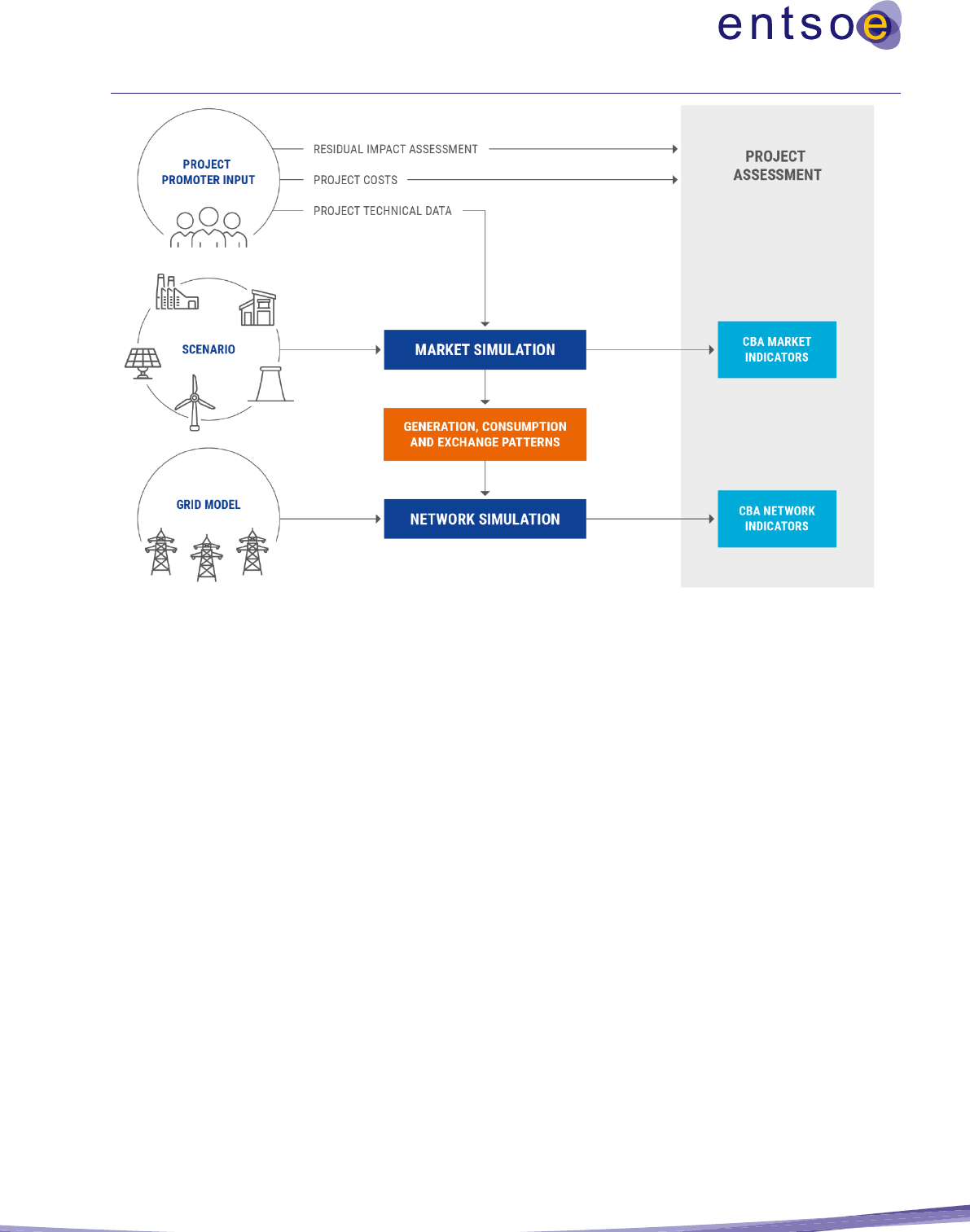
34
Figure 3: Schematic project assessment process. Whereas ‘CBA market indicators’ and ‘CBA network indicators’ are the direct
outcome of market and network studies, respectively, ‘project costs’ (see 5.10 and 511) and ‘residual impacts’ (see 5.13, 5.14
and 5.15) are obtained without the use of simulations.
3.2 General assumptions
This section provides general guidance on the assessment of projects. It provides guidelines for the
clustering of investment, the computation of transfer capability, the consideration of geographic scope, and
the calculation of a net-present value on the basis of the (monetised) indicators.
3.2.1 Clustering of investments
In some cases, a group of investments may be necessary to develop transmission capacities (i.e., one
investment cannot perform its intended function without the realisation of another investment). This process
is referred to as the clustering of investments. In this case, the project assessment is done for the combined
set of clustered investments.
When investments are clustered, it must be clearly demonstrated why this is necessary. Investments should
only be clustered together if an investment contributes to the realisation of the full potential of another
(main) investment. Investments that contribute only marginally to the full potential of the main investment
will not be clustered together.
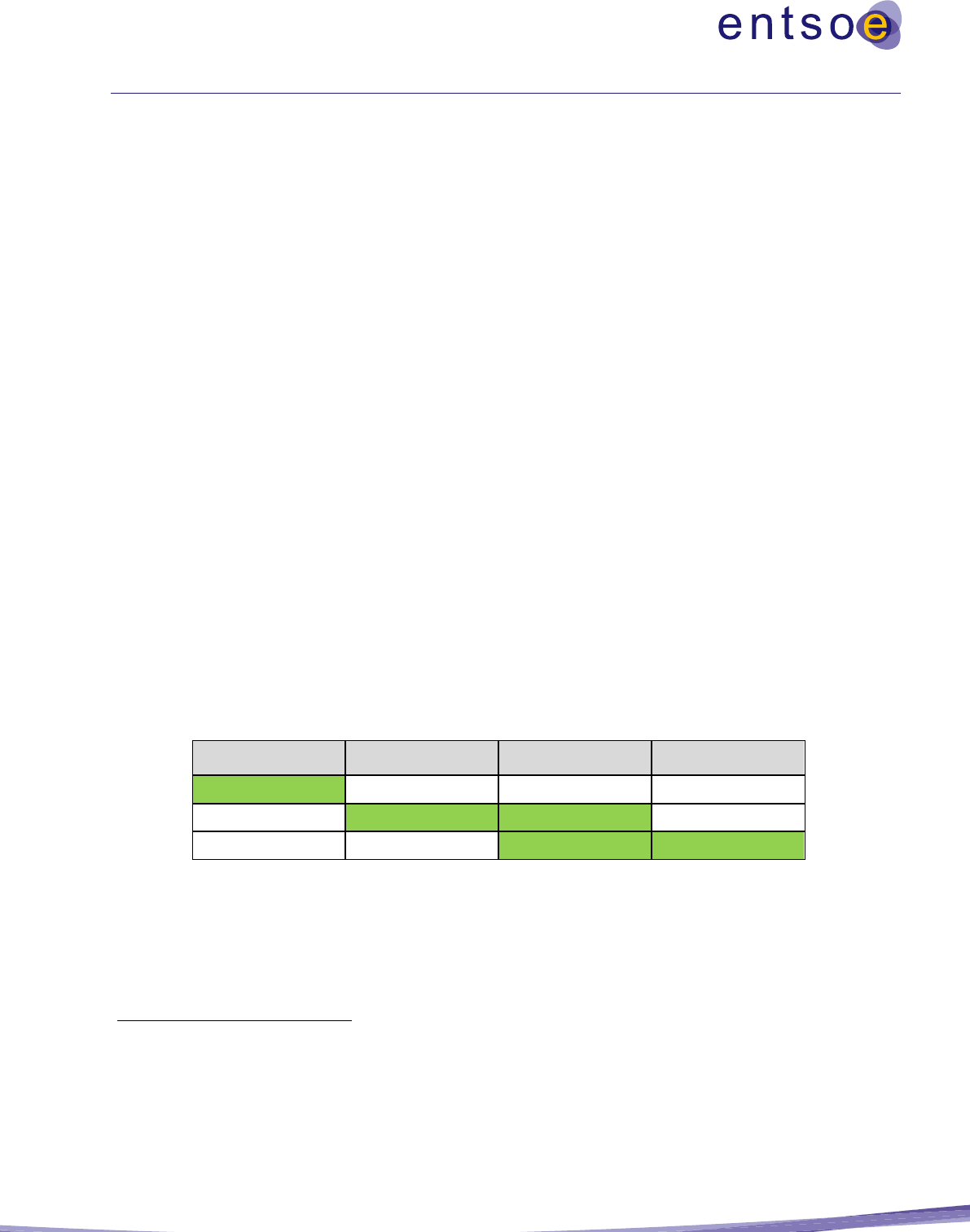
35
The full potential of the main investment represents its maximum transmission capacity in normal operation
conditions. When clustering investments, one main investment (e.g. an interconnector) must explicitly be
defined, which is supported by one or more supporting investments. A project that consists of more than
one investment is defined as a main investment with one or more supporting investments attached to it.
Note that competing investments cannot be clustered together.
Further limitations are as follows:
• Investments can only be clustered if they are at maximum of one stage of maturity apart from each
other, see Figure 4 below. This limiting criterion is introduced in order to avoid excessive clustering
of investments that do not contribute to realising the same function because they are commissioned
too far ahead in time.
• If an investment is ‘under consideration’, it can only be clustered with other investments in the
same stage, i.e. an investment under consideration cannot be clustered with an investment in
‘planned, but not yet in permitting’.
• If an investment is significantly delayed
12
compared to the previous TYNDP, it can no longer be
clustered within this project. To avoid a situation whereby investments are clustered when they are
commissioned far apart in time (which would also introduce a risk that one or more investments in
the project are never realised), a limiting criterion is introduced that prohibits the clustering of
investments that are more than one status away.
Figure 4 illustrates the categories of investments and which investments may be clustered. The categories
marked in green in each row can be clustered. For example, a main investment with status ‘permitting’ can
either be clustered together with investments that are ‘planned, but not yet in permitting’ (second row) or
‘under construction’ (third row).
Under
consideration
Planned, but not yet
in permitting
Permitting
Under
construction
Figure 4: Illustration of the clustering of investments
3.2.2 TOOT and PINT
There are two methods that are used to assess a project’s performance. These are illustrated in Figure 5 and
are described as follows:
12
The term ‘significant delay’ has to be seen as case-specific; in relation to all investments in that project, the investment with the earliest
commissioning date might be delayed further compared to that of the latest commissioning date. If two investments are more than 5 years apart,
they will be considered as significantly delayed and can no longer be clustered together. Exceptions can be made if the project promoter provides
a robust justification for the clustering.
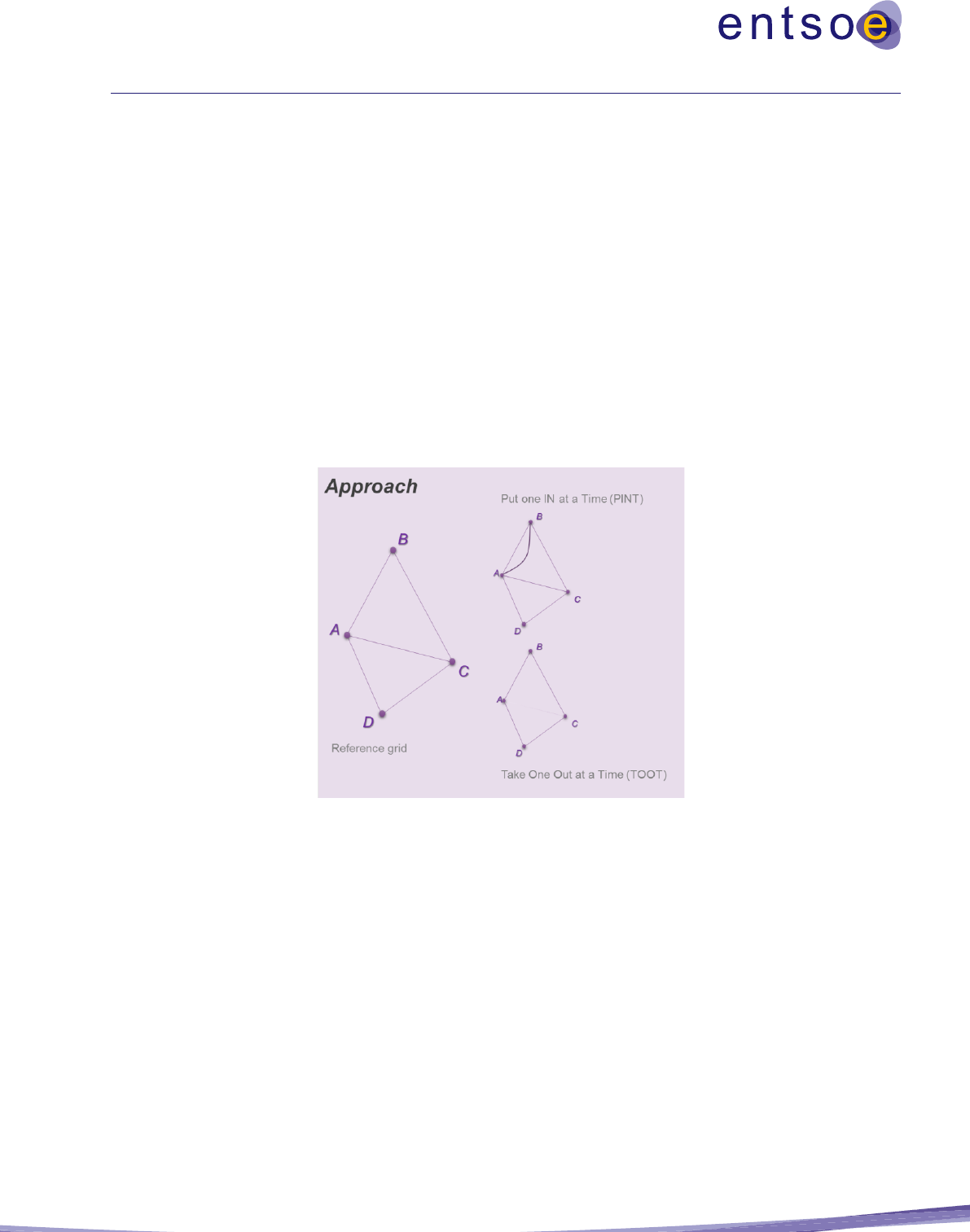
36
• Take Out One at the Time (TOOT) method:
The reference network represents a future target network in which all additional network capacity
is assumed to be in place (compared to the starting situation). The projects under assessment are
then removed from the future target network, one at a time, to evaluate the changes to each of the
indicators.
• Put IN one at the Time (PINT) method:
The reference network represents the initial state of the network without the projects under
assessment. The projects under assessment are then added to the reference network, one at a time,
to evaluate the changes to each of the indicators.
Projects that are ‘under consideration’ are considered non-mature and, therefore, have to be excluded from
the reference grid. These projects are assessed using the PINT approach, regardless of their position
regarding any additional criteria.
Figure 5: Illustration of TOOT and PINT approaches
The TOOT and PINT methods are to be applied consistently for both market and network simulations.
The TOOT method provides an estimate of the benefits for each project as if it were the last to be
commissioned; i.e. it is evaluated as part of the whole forecasted network. The advantage of this analysis
is that every benefit brought by each project is assessed together, without considering the order of projects.
Hence, this method facilitates assessment at the aggregated TYNDP level, with the future power system
and the evolution of every future network being considered.
For the PINT method, the reference network is clearly defined by the network model that is used; for market
simulations, the reference network considers the exchange capacities between the defined market zones,
including the additional capacity brought by the projects included in the grid. The PINT assessment is then

37
applied ‘on top’ of all projects assessed using the TOOT methodology and thus provide an estimation of
benefits for each project as if it were commissioned after all TOOT projects but is the first and only one to
be commissioned compared to all PINT projects.
In general, the application of the TOOT approach has the potential to underestimate the benefits of projects
because all project benefits are calculated under the assumption that the project is the final (marginal)
project to be realised. However, the application of the PINT approach has the potential to overestimate the
benefit of projects (compared to all other PINT projects) because all of the projects’ benefits are calculated
under the assumption that the project is the first project to be realised (after all TOOT projects have been
realised). Project benefits are generally, but not necessarily always, negatively affected by the presence of
other projects (i.e. if one project is built, a second one will have lower benefits). This effect is generally
strongest when two (or more) projects are constructed to achieve a common goal across the same boundary,
although it may also be present when projects are constructed along different boundaries.
Multiple applications of TOOT/PINT
For interdependent projects, the strict application of the TOOT or PINT methods may not fully reflect the
benefits of the projects. Therefore, in addition to the project benefits calculated using the strict application
of the TOOT or PINT methods, the benefits arising from the realisation of other projects on the same
boundary can be calculated (i.e. multiple TOOT or PINT). When the multiple TOOT or PINT methods (or
a combination of both) are applied, a detailed description of the sequence of projects must be given.
It should be noted that the reference for the second, third, etc. project in the sequence of the multiple
TOOT/PINT needs to be taken correspondingly. Whereas the first project in the sequence can be assessed
and compared against the reference grid (no change compared to the TOOT/PINT method as described
above), the reference for the second project should be such that the first project has been taken out (for
TOOT) or put in (for PINT). The third project needs to be assessed against the situation as defined by the
second step and so on.
Example for three interdependent TOOT projects:
Project number
Commissioning date
1
2021
2
2022
3
2024
o project 3: assessment against the reference grid by taking the project out.
o project 2: assessment against the situation with project 3 already taken out.
o project 1: assessment against the situation with project 3 and project 2 already taken out.

38
3.2.3 Transfer capability calculation
There are two concepts of transfer capability, namely: Net Transfer Capacity (NTC) and Grid Transfer
Capacity (GTC). NTC that this Guideline refers to is related to the potential for market exchanges of
electricity resulting in a power shift of dispatch from one bidding zone to another, and GTC is related to
physical power-flows that can be accommodated by the grid.
Net Transfer Capacity
The NTC reflects the ability of the grid to accommodate a market exchange between two neighbouring
bidding areas. An increase in NTC (ΔNTC) can be interpreted as an increased ability for the market to
commercially exchange power, i.e. to shift power generation from one area to another (or similarly for
load
13
). The physical power flow that is the result of this power shift may or may not directly flow across
the border of the two neighbouring bidding areas in its entirety, but may or may not transit through third
countries. The increase in the ability to accommodate market exchanges as a result of increasing physical
transmission capacity may, therefore, be different from the capability of the grid to transport physical power
across the border.
As the exchanges between bidding zones result in power-flows making use of the transport capacity across
the different boundaries they impact, an increase in GTC across a specific boundary is illustrative, ceteris
paribus,
14
of the increased exchange capability between these bidding zones.
Note that while the concept of NTC calculations in the context of long-term studies is similar to the
operational calculation of NTC values on borders, the concept of NTC, as defined for the purpose of long-
term planning studies, may show some differences in the sense that the approaches may not consider the
same operational considerations to ensure a safe and reliable operation of the system. The NTC values
reported in long-term studies are calculated under the ‘ceteris paribus’ assumption that nothing else in the
system changes (e.g. generation and load in neighbouring zones, RES fluctuations, loop flows) and,
therefore, does not have an impact on the calculated power shift made possible by the project (i.e. which
equals market exchange). In the TYNDP, the assumed utilisation of the additional GTC delivered by a
project will be reported in terms of the ability for additional commercial exchanges (i.e. ΔNTC) between
the bidding zones that define the boundary in question. Note that the ΔNTC is directional, which means
that values might be different in either direction of the commercial power-flow across a boundary.
ΔNTC is calculated using network models by applying a generation power shift
15
across the boundary under
consideration. This figure applies to the year-round situation (i.e. 8,760 hours) of how the generation power
shift affects the power-flow across the boundary under analysis. Calculating an ΔNTC value generally
results in a different value for each simulated time step of the year under consideration. This year-round
13
Wherever the text refers to ‘power shift’, both the ‘load shift’ and the ‘generation shift’ can be applied.
14
‘Ceteris paribus’ acknowledges that in actual system operations, one single boundary is not exclusively influenced by only the exchanges
between the bidding zones it relates to. The physical flow on the boundary can also be influenced by exchanges between other bidding zones
which, for example, cause loop or transit flows. These influences are not considered when calculating the increased NTC delivered by a project in
the context of this methodology.
15
It should be mentioned that the methodology on how the generation power-shift is applied can have a significant impact on the results and must
be clearly explained in the respective study. A consistent approach for the generation power shift must be applied for all assessments. The power
shift method(s) are to be defined in the Implementation Guideline and reported on the project sheets.

39
situation should be reflected in the load flow analysis either via a simulation of each individual time step
or via a simulation of a set of points in time that are representative of the year-round situation. The annual
delta NTC that is reported corresponds to the 70th percentile of the delta NTC duration curve (i.e. the value
is reached for at least 30% of the year). This is illustrated in Figure 6. In the event the reference NTCs used
in the market simulations are time-dependent (e.g. seasonal values are used), the calculated delta NTCs
could also be time-dependent, e.g. obtaining a different value for each season rather than a single annual
NTC.
Figure 6: Duration curve of ΔNTC in one direction (blue) with 70th percentile (red): the reported ΔNTC at the 70th percentile
needs to be reached at least 30% of the time – to the right of the red line.
The calculation of the ΔNTC is based upon a reference network model in line with the scenario considered.
As ΔNTC is the result of the possible power shift, the figure may differ between scenarios.
A detailed example of how the ΔNTC on one time step can be calculated is given in the Implementation
Guideline for the respective TYNDP.
Reporting on transfer capability
The impact on transfer capability must be reported on at the investment level for each project. This means
that the reporting must be done for each investment and also for the project as a whole. In the case of a
project with a cross-border impact, the figures to be reported are the ΔNTC of the project and the
contribution of the investment(s). For an internal project, ΔNTC must be reported
16
. In any case, for each
project it must be clearly displayed whether a cross-border transfer capacity, an internal transfer capacity,
or a combination of both types of transfer capacities is provided.
16
In case an internal project has a cross-border impact, the ΔNTC values have to be reported.

40
The method used to perform the generation power shift has to be reported in the respective study, and the
same method must be applied in a clear and consistent manner for all projects under assessment.
3.2.4 Geographical scope
The main principle of system modelling is to use detailed information within the studied area and a
decreasing level of detail outside the studied area. As a minimum requirement, the study area should cover
all MS and third countries on whose territory the project shall be built, all directly neighbouring MS, and
all other MS significantly impacted by the project.
17
To consider the interaction of the pan-European
modelled system in the market studies, exchange conditions with non-modelled countries will be fixed for
each of the simulation time steps based on a global market simulation.
18
Practically, the market model
should cover all European countries in addition to any third countries that host the assessed project. For
network analysis, each synchronous zone relevant for the project should be modelled (generally, this means
the synchronous zone in which the project is located; for HVDC projects between different synchronous
areas, all synchronous areas should be modelled, except for third countries).
Project appraisal is based on analyses of the global (European) increase of welfare.
19
This means that the
goal is to bring up the projects that are best for the European power system and, therefore, for European
society. Therefore it might be necessary to reduce the CBA results only to EU MS by excluding costs and
benefits located in third countries (non-EU MS). A detailed overview of the used perimeter applied for both
the simulation and the CBA evaluation needs to be given within the study specific Implementation
Guidelines. The defined perimeter has to fulfil the requirement to show what impact a project has on the
EU MS
20
. Separate from this possible split of costs and benefits, all results always need to also be given for
the full modelling perimeter.
3.2.5 Investment value calculation
The value of an investment is calculated using the discounted cash flow method. This method considers the
timing of costs and benefits and recognises that the value of money changes over time, which is often
referred to as the time value of money. The assumption is that the value of money changes at a constant
annual rate, referred to as the discount rate. The future values of both costs and benefits can then be
represented (or discounted) to present values using the discount rate.
The present value (PV) of a future cost or benefit (referred to as FV) in a given time period n, using a
discount rate of r per annum, is described by the following formula:
17
Annex V, §1 Regulation (EU) 2022/869
18
Within ENTSO-E, this global simulation would be based on a pan-European market data base.
19
Some benefits (socio-economic welfare, CO
2
…) may also be disaggregated on a smaller geographical scale, like a member state or a TSO area.
This is mainly useful in the perspective of cost allocation and should be calculated on a case-by-case basis, taking into account the larger
variability of results across scenarios when calculating benefits related to smaller areas. In any cost allocation, due regard should be paid to
compensation moneys paid under ITC (which is article 13 of Regulation 714 (see also Error! Reference source not found. for caveats on
Market Power and cost allocation).
20
It is considered that societal impacts based on CO
2
emissions will occur independent of where the CO
2
is emitted. Therefore the B2 indicator
might be still considered based on the whole perimeter, while other indicators are reduced just to the EU perimeter.

41
The main methods used to represent the value of an investment as a single value are Net Present Value
(NPV) and Benefit-to-Cost Ratio (BCR). Both methods assess the viability of the investment, and where
there are a number of competing investments they are used to facilitate a comparison of competing
investments where consistent assumptions are applied.
The NPV of an investment is the difference between the present value of benefits (i.e. cash inflows) and
the present value of costs (i.e. cash outflows) over the economic life of the investment. A viable investment
is usually indicated by a positive NPV, i.e. the present value of benefits is greater than the present value of
costs.
The NPV of the investment assessed over the assessment period of T years is described by the following
formula:
Where t0 calculates as the commissioning minus the year of the study and T is defined as the assessment
period added to t0.
The BCR of an investment is the ratio of the present value of benefits to the present value of costs. A viable
investment is usually indicated by a BCR greater than one, i.e. the present value of benefits is greater than
the present value of costs.
The BCR of the investment is calculated over the assessment period of T years using the following formula:
To enable the consistent calculation of either the NPV or BCR for an investment, a consistent set of
assumptions must be applied. Given that both methods use the same calculations to determine the present
value of benefits and costs, the assumptions apply equally to both methods.
The key assumptions are as follows:
The assessment period defines the period of time over which the investment will be evaluated. This may
be different to the useful life of the investment’s assets and represents the period over which it is reasonable,
given the uncertainty, to expect value to be attributed to the investment. For the purposes of this guideline,
the assessment period is 25 years.

42
Values are represented as real and constant values. This means that no inflation is considered and, therefore,
no forecasts for future inflation are necessary. It also means that values are taken as fixed throughout the
assessment by assuming constant year-of-study values. The year-of-study is taken as the year of the
TYNDP, i.e. 2024 for the TYNDP 2024. The impact of taxation is not considered in the project assessments,
so the values are represented as pre-tax values.
The discount rate used to calculate the NPV can differ between countries; however, for a fair assessment
across projects, a common discount rate is required. For the purposes of this guideline, the discount rate
should be given as a real value. The real discount rate to be used is 4% per annum.
Future values are to be discounted to a common point in time, which is the year of the TYNDP, also referred
to as the year-of-study above.
The forecasted costs and benefits for each investment are to be represented annually.
The year of commissioning is the year that the investment is expected to come into first operation.
The inception costs are to be aggregated and represented in the commissioning year of the investment as a
single value.
Further capital costs incurred to sustain the investment during its lifetime are to be represented in real and
constant year-of-study values in the year that they occur.
The benefits are accounted for from the first year after commissioning. To evaluate projects on a common
basis, benefits should be aggregated across the years, as follows:
• For years from the first year after commissioning (i.e. the start of benefits) to the first mid-term: extend the
first mid-term benefits backwards;
• For years between different mid-term, long-term and very long-term (if any): linearly interpolate benefits
between the time horizons; and
• For years beyond the farthest time horizon: maintain benefits of this farthest time horizon.
To assess a project that is comprised of multiple investments, the annualised benefits, losses and operational
costs for the project are accounted for from the commissioning of the latest investment, thus the
commissioning of the complete project.
The residual value of the project at the end of the assessment period should be treated as having zero value.
3.3 Assessment framework
The assessment framework laid out in this Guideline is consistent with Article 11 and Annexes IV and V
of the Regulation, and describes the structure used to differentiate the range of indicators that comprise the
project assessment.
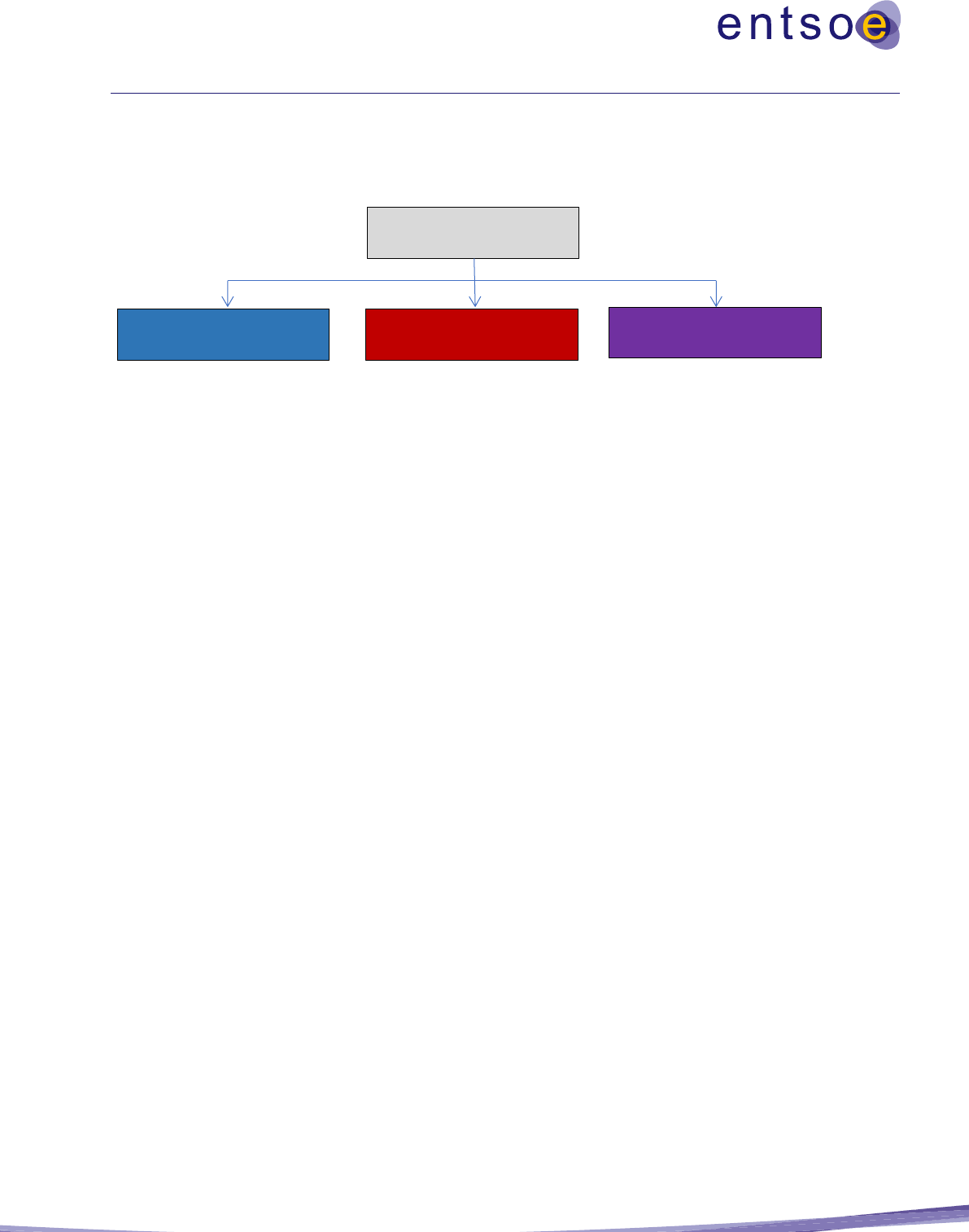
43
The assessment framework comprises three main categories – costs, benefits and residual impacts – as
illustrated in Figure 7. Within each of the three categories, there are a number of separate and distinct
indicators that together represent the category. The composition of each of the categories is described in
detail in Chapter 5.
Figure 7: Overview of the main categories of CBA indicators
Benefits describe the positive contributions made by the project. The formalised indicators that comprise
the benefits are supported by detailed methodologies that are captured in their corresponding sections in
Chapter 5. Note that projects may also have a negative impact on some benefit indicators, in which case
negative benefits are reported.
Costs describe the inception cost of the project or investment, i.e. CAPEX and the operating costs that
incurred throughout the investment’s lifecycle, i.e. OPEX. The CAPEX cost typically refers to the inception
cost of the project and would also include the costs of implementing mitigation measures that address
environmental and social constraints.
Residual impacts describe the impacts of investments that are not addressed by any of the identified
mitigation measures that are contained within the cost category (typically as CAPEX). This ensures that all
measurable costs associated with projects or investments are considered, and that no double-accounting
occurs between any of the indicators.
3.4 Non-mature indicators
In some instances, there are costs or benefits that are relevant for a CBA, but it might not be possible to
assess them at a pan-European level. This is the case when common applicable and on pan-European level
agreed datasets are not available or when the methodological description has not achieved a sufficient level
of maturity. However, for completeness reasons and to maintain consistency, all indicators, including the
here mentioned non-mature indicators, are also displayed in this Guideline in Chapter 5, with a clear
information about their non-mature status.
Although the Pan-European nature of these indicators is recognised, it is acceptable to assess them relying
on a regional, or even national, perimeter to deal with their inherent complexity. In that case, additional
information on the used tools, datasets, assumptions and a detailed description of the used methodology
needs to be given within the respective study.
Project Assessment
Benefits
Costs
Residual Impacts

44
4 Concluding remarks
This guideline for the CBA of grid development projects was prepared by ENTSO-E in compliance with
the requirements of the EU Regulation (EU) 2022/869. This guideline is the fourth version of the document
produced by ENTSO-E and is built upon the 3
rd
CBA Guideline, which was the result of an extensive
consultation process.
The document is a general guide to assist in the assessment of planned projects included in ENTSO-E’s
TYNDP. It describes the common principles and procedures for performing the analysis of costs and
benefits for projects using network and market simulation methodologies. Following Regulation (EU)
2022/869 on guidelines for trans-European energy infrastructure, it also serves as the basis for a harmonised
assessment of PCIs at the European Union level.
A multi-criteria approach is used to describe the indicators associated with each project. To ensure a full
assessment of all transmission benefits, some of the indicators are monetised, whereas others are quantified
in their typical physical units (i.e. tons or GWh). The set of common indicators contained in this Guideline
form a complete and solid basis for project assessment across Europe, both within the scope of the TYNDP
as well as for project portfolio development in the PCI selection process.
This CBA Guideline is drafted using a modular approach. The purpose of the modular approach is to enable
more efficient updates of the Guideline by allowing stakeholders to better focus on specific content without
necessarily impacting the whole document. This recognises that the Guideline is an evolving and living
document that we endeavour to continually improve to meet the needs of our stakeholders.
The following sections give more concrete information on the single indicators and additional specific
context.
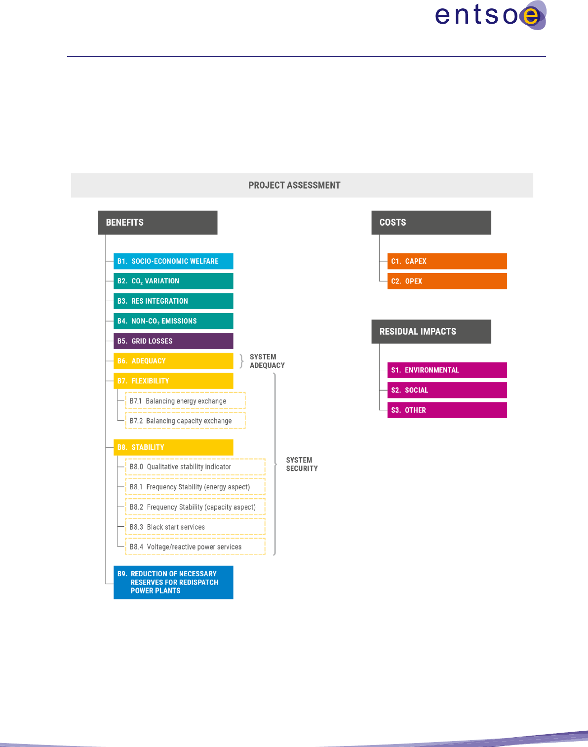
45
5 Benefits, costs and residual impacts
The project assessment is conducted using the benefit, cost and residual impact indicators described in this
Guideline. Although the benefits should be given for each study scenario (e.g. the TYNDP scenarios), costs
and residual impacts are seen as scenario independent indicators.
The main project assessment categories are illustrated in Figure 8:
Figure 8: Illustration of the project assessment framework categories

46
The indicators have been selected on the following bases:
• They facilitate the description of the project costs and benefits in terms of the EU network
objectives. These EU network objectives are:
o to ensure the development of a single European grid, enabling EU climate policy and
sustainability objectives (i.e. RES, energy efficiency, CO
2
);
o to guarantee SoS;
o to complete the internal energy market, especially through a contribution to increased SEW
and;
o to ensure system stability.
• They provide a measurement of a project’s costs and feasibility (especially environmentally and
socially, as indicated by the residual impact indicators).
• They are as simple and robust as possible. This facilitates simplified methodologies where practical
to do so.
The project assessment should reflect the average transfer capacity contribution of the project. The
contribution to transfer capacity is time and scenario dependent, but a single or seasonal value should be
reported for clarity reasons. A characterisation of a project is provided through an assessment of the
directional ∆NTC increase and the impact on the level of electricity interconnection, relative to the installed
production capacity in the MS.
21
For those countries that have not reached the minimum interconnection
ratio, as defined by the EC, each project must report the contribution to achieve this minimum threshold.
However, the interconnection targets must not be considered as a technical criteria and therefore have to be
treated differently from the indicators given in section 5 in order to avoid any double accounting.
The increased transfer capacity contribution and costs are given per investment, whereas the benefit
indicators and residual impact indicators are provided at the project level.
For some of the indicators, it is not yet possible to deliver a mature methodology to assess them on a Pan-
EU level. This 4th CBA Guideline introduces five non-mature indicators:
• B7.1: Balancing energy exchange (aFRR, mFRR, RR);
• B7.2 Balancing capacity exchange/sharing (aFRR, mFRR, RR);
• B8.1: Frequency Stability;
• B8.2: Black start services; and
• B8.3: Voltage/reactive power services
The benefit indicators are described as follows:
21
Regulation (EU) 2018/1999 of the European Parliament and of the Council of 11 December 2018 on the Governance of the Energy Union and
Climate Action establishes, in article 23 (a), that ‘…the level of electricity interconnectivity that the Member State aims for in 2030 in
consideration of the electricity interconnection target for 2030 of at least 15 % …’

47
B1. Socioeconomic welfare (SEW from wholesale energy market integration),
22
in the context of
transmission network development, is the sum of the short-run economic surpluses of electricity
consumers, producers and transmission owners. The indicator reflects the contribution of the
project or investment to increasing transmission capacity, making an increase in commercial
exchanges possible so that electricity markets can trade power in a more economically efficient
manner. It is characterised by the ability of a project or investment to reduce (economic or physical)
congestion. Under multi-sectorial market coupling, the indicator can be augmented to the global
SEW comprising the individual contributions of the different sectors.
B2. Additional societal benefit due to CO
2
variation is the change in CO
2
emissions produced by the
power system due to the project. It is a consequence of changes in generation dispatch and the
unlocking of renewable generation potential. This indicator is directly linked to the EU’s climate
policy goal of reducing greenhouse gas emissions by at least 55% by 2030 relative to 1990 levels.
As CO
2
emissions are the main greenhouse gas produced by the electricity sector, they are
displayed as a separate indicator, and its monetary benefit is described using societal costs for
carbon.
B3. RES integration defines the ability of the power system to connect new RES generation, unlock
existing and future ‘renewable’ generation, and minimise the curtailment of electricity produced
from RES.
23
The RES integration indicator is linked to the EU 2030 goal of increasing the share of
RES to 32% of overall energy consumption.
B4. Non-direct greenhouse emissions refer to the change in non-CO
2
emissions (e.g. CO
X
, NO
X
, SO
X
,
PM 2, 5, 10) in the power system due to the project. They are a consequence of changes in
generation dispatch and the unlocking of renewable generation potential.
B5. Grid losses in the transmission grid is the cost of compensating for thermal losses in the power
system due to the project. It is an indicator of energy efficiency
24
and is expressed as a cost in euros
per year.
B6. Security of supply: Adequacy characterises the project's impact on the ability of a power system
to provide an adequate supply of electricity to meet demand over an extended period of time.
Variability of climatic effects on demand and RES production is considered.
B7. Security of supply: Flexibility characterises the impact of the project on the ability to exchange
balancing energy in the context of high penetration levels of non-dispatchable electricity
generation. Balancing energy refers to products such as Replacement Reserve (RR), manual
Frequency Regulation Reserve (mRR) and automatic Frequency Regulation Reserve (aFRR).
Exchanging/sharing balancing capacity (i.e. RR, mFRR and aFRR) that requires guaranteed or
22
The reduction of congestions is an indicator of social and economic welfare assuming equitable distribution of benefits under the goal of the
European Union to develop an integrated market (perfect market assumption). The SEW indicator focuses on the short-run marginal costs.
23
This category corresponds to B3: Methodology for RES Integration Benefit .
24
This category contributes to B5: Methodology for Variation in Grid Losses Benefit

48
reserved cross-zonal capacity is also considered. This indicator is considered as non-mature where
further development is needed.
B8. Security of supply: Stability characterises the project’s impact on the ability of a power system to
provide a secure supply of electricity as per the technical criteria. This indicator (except of the
qualitative part) is considered as non-mature where further development is needed.
B9. Redispatch Reserves or Reduction of Necessary Reserves for Redispatch Power Plants
describes a project’s impact on the required levels of contracted redispatch reserve power plants by
assessing the maximum power of redispatch with and without the project. A prerequisite for this
indicator is the use of redispatch simulations.
The costs indicators are described as follows:
C1. Capital expenditure (CAPEX). This indicator reports the capital expenditure of a project, which
includes elements such as the cost of obtaining permits, conducting feasibility studies, obtaining
rights-of-way, ground, preparatory work, designing, dismantling, equipment purchases and
installation. CAPEX is established by analogous estimation (based on information from prior
projects similar to the current project) and by parametric estimation (based on public information
about the cost of similar projects). CAPEX is expressed in euros.
C2. Operating expenditure (OPEX). OPEX defines the annual operating and maintenance expenses
associated with the project or investment. OPEX is expressed in euros per year.
Residual impact indicators refer to the impacts that remain after impact mitigation measures have been
taken. Hence, impacts mitigated by additional measures should no longer be listed in this category. The
indicators are defined as follows:
S1. Residual Environmental impact characterises the (residual) project impact on the environment,
as assessed through preliminary studies, and aims to provide a measure of the environmental
sensitivity associated with the project.
S2. Residual Social impact characterises the (residual) project impact on the (local) population
affected by the project, as assessed through preliminary studies, and aims to provide a measure of
the social sensitivity associated with the project.
S3. Other impacts provide an indicator of all other impacts of a project.
Although ENTSO-E intends to monetise as many of the indicators as possible, in some cases the required
data are not always available (e.g. detailed emission prices per fuel type for non-CO
2
calculations). ENTSO-
E seeks to deliver a uniform and objective CBA assessment and is reluctant to publish results if their
uniformity and/or objectivity cannot be guaranteed. In such cases, it is more useful to publish indicator
results in their original units than to unilaterally decide on their monetary value in an arbitrary manner.

49
It should be noted that for those indicators that require monetisation, the euro values are to be represented
as real and constant values. This means that no inflation is considered and, therefore, no forecasts for future
inflation are necessary. It also means that values are taken as being fixed throughout the assessment by
assuming constant year-of-study values. The year-of-study is taken as the year of the TYNDP, i.e. 2024 for
the TYNDP 2024. The impact of taxation is not considered in the project assessments, so the values are to
be represented as pre-tax values.
The table below provides an overview of the status, regarding monetisation, of the benefit indicators
included in this 4
th
CBA Guideline:

50
Table 2: Overview of the status of indicator monetisation
Indicator
Unit
Monetisation status
Document location
B1. SEW
€/yr
Monetised by definition
B1: Methodology for
Socioeconomic Welfare
Benefit
B2. CO
2
emissions
Tons/yr
and €/yr
Comprises two parts: (1) Fully monetised in B1,
where the effects of CO
2
emissions are
monetised and reported as additional
information under indicator B1. (2) Related to
the additional societal value, which is not
monetised under B1.
Political CO
2
reduction targets are
formulated as percentages of values,
expressed in tons per year. The monetary
effect is the topic of ongoing political
debate. Therefore, the CBA Guideline
requires that CO
2
emissions are reported
separately (in tons).
B2: Methodology for
Additional Societal benefit due
to CO2 variation
B3. RES integration
MW or
MWh/yr
Fully monetised under B1, where the effects of
RES integration on SEW, due to the reduction
of curtailment and lower short-run variable
generation costs, are monetised and reported as
additional information.
Political RES integration goals are
formulated and expressed in MW. The
monetary effect (in addition to B1, B2)
cannot be monetised objectively.
Therefore, the CBA Guideline requires
that RES integration is reported separately
(MW or MWh/yr).
B3: Methodology for RES
Integration Benefit
B4. Non-CO
2
emissions
Tons/yr
Not monetised
B4: Methodology for Non-
Direct Greenhouse Emissions
Benefit
B5. Grid losses
MWh/yr
Monetised using hourly marginal costs from the
market simulations per price zone.
B5: Methodology for Variation
in Grid Losses Benefit
B6. SoS: Adequacy
MWh/yr
Monetised. Is dependent on availability of
VOLL-values. Additional adequacy margin
may be conservatively monetised using
investment costs in peaking units (provided
figures are available).
B6: Methodology for Security
of Supply: Adequacy to Meet
Demand Benefit
B7. SoS: Flexibility (balancing
energy exchange)
Ordinal scale
Not monetised.
Not monetised at present because of the
unavailability of quantitative models. First
development is to provide quantitative
model results.
B7: Methodology for Security
of Supply – System Flexibility
Benefit

51
B8. SoS: Stability
Ordinal scale
Not monetised.
Not monetised at present because of the
unavailability of quantitative models. First
development is to provide quantitative
model results.
Section 5.8:
B8: Methodology for
Security of Supply: System
Stability Benefit
B9. Redispatch Reserves or
Reduction of Necessary
Reserves for Redispatch
Power Plants
Redispatch Reserves
€/yr
Monetised using actual costs for allocation of
redispatch reserves
This indicator is optional and can only be
achieved when the SEW has been
calculated using redispatch simulations
Section 5.9:
Reduction of Necessary
Reserve for Redispatch Power
Plants (B9)

52
5.1 B1: Methodology for Socioeconomic Welfare Benefit
Introduction
In power system analysis, SEW is typically defined as the sum of the short-run economic surpluses of
electricity consumers, producers and transmission owners (congestion rent). Transmission network
projects, or investments, have an effect on the sum and the distribution of these surpluses. Investment in
transmission capacity generally increases the total sum of the individual surpluses by enabling a larger
proportion of demand to be met by cheaper generation units that were not available before because of a
transmission bottleneck.
These surplus effects are only one part of the overall economic benefit provided by transmission
investments that stem from wholesale energy market integration and do not capture other transmission-
related benefits as described by the other indicators, as given in this guideline.
Calculations within the respective studies (e.g. the TYNDP) should be based on a set of scenarios, which
are designed to represent future conditions with regard to generation and demand. The contents of the
scenarios are carefully determined and consider a coherent set of assumptions with regard to possible
developments in generation and load. This allows the marginal benefits of a transmission project to be
assessed against a 'static' reference framework. In reality, the transmission project actually alters the
reference framework itself – albeit with a (frequently significant) time delay. Considering that these longer-
term effects make the modelling challenge considerably more complex and decrease the robustness of
results, the strength of an approach based on reporting the marginal differences in short-run surplus lies in
its unambiguity.
Indicator definition:
• Definition: In power system analysis, SEW is typically defined as the sum of the
short-run economic surpluses of electricity consumers, producers and transmission
owners (congestion rent). In a multi-sector CBA project assessment, the SEW
corresponds to the global SEW.
• Relevance: This indicator gives a direct measure for the monetary benefit and is
therefore of great relevance for the CBA.
Indicator calculation:
• Model: Market simulations, Redispatch simulations; based on a system cost
comparison with/without the project.
• Quantitative measure: this indicator is directly given in monetary values.
• Monetisation: per definition monetised and given in €/year
Interlinkage to other CBA indicators:
• B2, B3, B6

53
In the presence of sector coupling, the concept of SEW can be applied to multiple sectors. In this regard,
those sectors represent different markets for different energy carriers e.g. electricity, hydrogen, methane,
etc. Moreover, their contributions constitute the overarching global SEW that covers the entire energy
system and captures cross-sectorial benefits. It is composed into the individual aforementioned standard
surpluses and contributions stemming from the interlinkage of the involved sectors that are defined as cross-
sector rents. They can be used to decompose the global SEW in its sectorial counterparts by attributing the
benefits to the involved sectors. Their calculation is optional and can be considered an augmented and
alternative approach to the standard economic welfare decomposition. Table 3 shows the different options
for the SEW calculation depending on the project assessment type.
Table 3: Options for SEW calculation under multi-sector or single sector project assessments
Indicator
Multi Sector Assessment
Single Sector Assessment
Global SEW
X
SEW for electricity
X
25
X
Methodology
The TYNDP reports changes to economic surpluses as a result of transmission projects, i.e. 'deltas' between
situations with and without the project under consideration. It unambiguously reports the marginal change
to the total economic surplus in the event of building a transmission project, without the need to further
consider secondary consequences, which are usually not merely the result of constructing the transmission
project but rather the result of (related and unrelated) further (political) decisions.
To calculate the change in short-term economic surplus, a perfect market is assumed. The perfect market
assumes all market participants have equal access to information, no barriers to entry or exit, and no market
power.
In general, two different approaches can be used for calculating the variation in SEW:
• The generation cost approach, which compares the generation costs with and without the project
for the different bidding areas; and
• The total surplus approach, which compares the producer and consumer surpluses for both bidding
areas, in addition to the congestion rent between them and potentially the cross-sector rents
stemming from the interlinkage between the sectors, with and without the project.
26
25
Calculation is only possible under the Total Surplus (TS) approach. This could be done in combination with the introduced cross-sector rent
component.
26
More details about how to calculate surplus are provided in
B1: Methodology for Socioeconomic Welfare Benefit. Further calculation details under multi-sector project assessment will be given in the
respective TYNDP implementation guidelines.
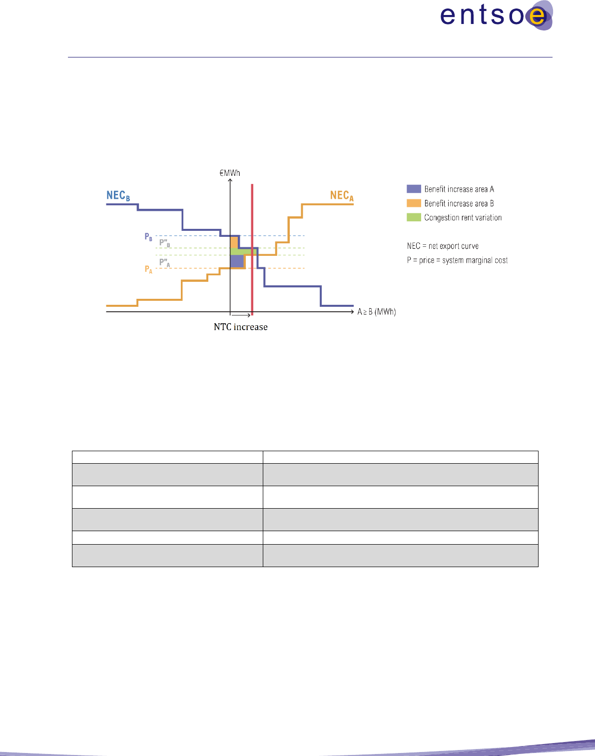
54
When measuring the benefits of transmission investments under the assumption of perfectly inelastic
demand, the change in SEW is equal to the reduction in total variable generation costs. Hence, if demand
is considered as perfectly inelastic to price, both methods will yield the same result. This metric values
transmission investment in terms of saving total generation costs as a project that increases the commercial
exchange capability between two bidding areas allows generators in the lower priced area to export power
to the higher priced area, as shown in Figure 9.
Figure 9: Illustration of benefits due to NTC increase between two bidding areas -+
The new transmission capacity reduces the fuel and other variable operating costs and, hence, increases
total SEW. Total generation costs are equal to the sum of thermal generation costs (fuel plus CO
2
ETS
costs), and DSR costs. The different cost terms generally used in market simulations are shown in the Table
4: cost terms used in market simulations.
Table 4: cost terms used in market simulations
Cost terms in market simulations
Description
Fuel costs
Costs for fuel of thermal power plants (e.g., lignite, hard coal, natural
gas, etc.).
CO
2
-Costs
Costs for CO
2
-emissions caused by thermal fired power plants. Depends
on the power generation of thermal power plants and price of CO
2
.
Start-up-costs/Shut-down costs
These terms reflect the quasi-fixed costs for starting up a thermal power
plant to at least a minimum power level.
Operation and maintenance costs
Costs for operation and maintenance of power plants.
Demand Side Response (DSR) costs
Costs of DSR. DSR is the load demand that can be actively changed by a
certain trigger.
If demand is considered elastic, modelling becomes more complex. Most European countries are considered
to have price inelastic demand. However, there are a number of developments that appear to increase the
price elasticity of demand. These developments include smart grids and smart metering, as well as a
growing need for flexibility in order to accommodate the changing production technologies (i.e., more
renewables, less thermal and nuclear).

55
The choice of assumptions regarding demand elasticity and the methodology for the calculation SEW
benefit is left to ENTSO-E’s Regional Group to decide. There are two recognised approaches considering
greater flexibility of demand when assessing SEW, and these are listed below. The choice of the approach
needs to be decided within the respective study, e.g. based on the respective Implementation Guidelines.
In the first approach, demand is estimated through scenarios, which results in a reshaping of the demand
curve (in comparison with present curves) to model the future introduction of smart grids, electric vehicles,
etc. In this case, demand response is not elastic at each time step, but constitutes a shift of energy
consumption from time steps with potentially high prices to time steps with potentially low prices (e.g. on
the basis of hourly RES availability factors). The generation costs to supply a known demand are minimised
through the generation cost approach. This assumption simplifies the complexity of the model and,
therefore, the demand can be treated as a time series of loads that have to be met, while simultaneously
considering different scenarios of demand-side management.
The second approach introduce hypotheses regarding the level of price elasticity of demand. To do this,
there are two possible methods:
• Generation cost method:
Using the generation cost approach, price elasticity could be considered via the modelling of
curtailment as generators. The willingness to pay would then, for instance, be established at very
high levels for domestic consumers and at lower levels for a part of industrial demand.
• Total surplus method:
Using the total surplus method, the modelling of demand flexibility would need to be based on a
quantification of the link between price and demand for each hour, allowing a correct representation
of demand response in each area.
These methods are discussed in detail in the Annexes. Annex 6.4 addresses the generation cost method and
Annex II addresses the total surplus method.
Changes in SEW must be reported in euros per year (€/yr) for each project, for a given scenario and study
year. In addition to the overall SEW changes, the SEW changes that are the result of integrating RES and/or
variations in CO
2
-emissions must be reported separately as follows:
• Fuel savings due to integration of RES; and
• Avoided CO
2
emission costs.
Monetisation
This indicator is measured in €/yr and is, therefore, monetised by default.
The effects of CO
2
emissions, based on assumptions regarding emission costs, are monetised and reported
as additional information under indicator B1.

56
The effects of RES integration on SEW due to the reduction of curtailment and lower short-run variable
generation costs is monetised and reported as additional information under indicator B1.
Independent of the methodology used to calculate the SEW, the result will be given as a single value in €/yr
as received by the respective methodology (i.e. no summation of the values achieved by the different
methods) plus additional information on the RES and CO
2
impact on the SEW.
For cross-border projects, either the reduced generation costs/additional overall welfare or the combination
with redispatch costs are calculated. For projects that have no cross-border capacity impact, only the
redispatch methodology is used. The method used to calculate the SEW must always be reported.
Double-counting
The monetisation of RES and CO2 under this indicator has to be seen as supplementary information and
must not be added to the SEW figure. Furthermore, dependent on the methodology used for monetising the
RES part of this indicator (which has to be defined within the project-specific Implementation Guidelines),
the sum over the monetary part of RES and CO2 can exceed the total SEW delivered.
An overview of the different methods to calculate the SEW is given in Table 5.
Table 5: Reporting Sheet for this Indicator in the TYNDP.
Parameter
Source of Calculation
Basic Unit of
Measure
Monetary Measure
Level of Coherence
SEW: Reduced
generation costs/
additional overall
welfare
Market studies
(optimisation of
generation portfolios
across boundaries)
€/yr
per definition
monetary
European
SEW: Redispatch costs
Redispatch studies
(optimisation of
generation dispatch
within a boundary
considering grid
constraints)
€/yr
per definition
monetary
Regional/Project
promoter (PP) level
SEW: Reduced
generation cost/
additional overall
welfare + Redispatch
costs
Combination of both
market- and
redispatch-simulation
€/yr
per definition
monetary
Regional/PP level

57
5.2 B2: Methodology for Additional Societal benefit due to CO
2
variation
Introduction
As a signatory of the Paris Agreement, the European Union is committed to lower its carbon impact. In
November 2018, the EC presented its strategic long-term vision for a prosperous, modern, competitive and
climate-neutral Europe by 2050. This common goal aims to limit global warming and its harmful impact
on the world. The European electricity system is a significant contributor to CO
2
emissions. In this context,
grid development can play a role in modifying the level of carbon emissions. In particular, new
interconnector projects enable cheaper generators to replace more expensive plants with potentially higher
CO
2
emissions, leading to potentially lower CO
2
emissions.
To fully display the benefits of reducing CO
2
emissions due to a new project or investment, this indicator
is divided into two parts:
• Part 1 refers to the change in pure CO
2
27
emissions given in tons; and
27
All CO
2
values (in [t] and ETS costs) are considered being pure CO
2
without considering equivalents as coming from other emission types.
Indicator definition:
• Definition: This indicator gives the change in CO
2
emission due to a new project or
investment and is divided into two parts: the pure CO
2
emission in tons and
additionally the societal costs in €/year. Both measures have to be displayed.
• Relevance: The European electricity system is a significant contributor to CO
2
emissions. In this context, grid development can play a role in modifying the level of
carbon emissions. Due to the common goal to limit global warming and its harmful
impact on the world, both measures of CO
2
(absolute and monetary) are given.
Indicator calculation:
• Model: Market simulations, Network simulations, Redispatch simulations; based on
the CO
2
emissions comparison with/without the project.
• Quantitative measure: this indicator is for the first part given in tons
• Monetisation: the second part is monetised by the multiplication of CO
2
emissions [t]
and a defined factor [€/t]
Interlinkage to other CBA indicators:
• B1, B3, B5

58
• Part 2 refers to its monetisation. The monetary part of CO
2
is partly considered within SEW and
losses through the generation cost. The marginal cost for each power plant is the sum of the fuel
cost and the CO
2
market price. This CO
2
price, which is paid for by the producers, is the forecast
of the CO
2
price over the Emission Trading Scheme (ETS). Depending on the level of this market
price, the forecasted price signal may be too low to give a sufficient price signal to lead to the
investment level required to reach Europe’s climate goal.
Thus, to appropriately assess investments in accordance with the European objective of CO
2
emission
reduction, a specific indicator for monetising this additional impact is designed. For this purpose, the
variation in CO
2
emissions is valued at the appropriate level of a societal cost. This cost represents the effort
that should be made to reach the European climate-neutral goal.
Methodology
The CO
2
emissions are computed with and without the project. The variations that are considered for this
indicator are:
• Variations resulting from the change of generation plan; and
• Variations resulting from the change of losses volumes.
To avoid double accounting with the CO
2
variation already monetised into the SEW (B1) and the losses
(B5), changes in CO
2
emission are then multiplied by the difference between the CO
2
societal cost and the
ETS price used in the scenario. This benefit (B2) is to be added to the overall monetary benefit.
This is shown as follows:
Note: this formula only applies when the ETS costs are lower than the defined societal costs. If the ETS
costs are already above the societal costs, only the ETS costs are used, and this indicator does not bring
additional monetary benefit.
Example: for a hypothetical project from A to B
The impact of the project is described as follows:
• Impact on CO
2
emissions on the generation plan (using market simulations): -0.8 Mton/yr; and
• Impact on CO
2
emission of losses volume changes (using network simulations): +0.2 Mton/yr
Given that the ETS price in the scenario is 27 €/ton; and

59
Societal cost is taken as 163 €/ton
28
, the benefit is calculated as follows:
• B2 benefit = (0.8 – 0.2)*(163 – 27) = 81.6 M€/yr
Monetisation
The second part of this indicator is measured in €/yr and is, therefore, monetised by default.
The CO
2
cost used should be based on reputable scientific investigations and international studies. Because
of the expected spread of values that typically arise from different sources, the costs that are used can be
given as a range, e.g. by defining minimum, medium and maximum values, and should ideally be agreed
between the main stakeholders and reflect the most recent values as given by the EC. The values used for
the monetisation of this indicator have to be given within the study-specific Implementation Guidelines,
together with a link to the scientific and agreed study. The societal cost of carbon can represent two
concepts:
• The social cost that represents the total net damage of an extra metric ton of CO
2
emission due to
the associated climate change;
29
and
• The shadow price determined by the climate goal under consideration. It can be interpreted as the
willingness to pay for imposing the goal as a political constraint.
30
Double-counting
It is important to emphasise that this 'societal cost of CO
2
' is a different concept to the price of CO
2
that is
imposed on carbon-based electricity production, which may take the form of carbon taxes and/or the
obligation to purchase CO
2
emission rights under the ETS. The cost of the latter is internalised in production
costs and has a direct effect on SEW; hence, it is fully captured by indicators B1 and B5 (and also reported
as such alongside the B1 and B5 indicators). However, the cost of CO
2
imposed on electricity producers
does not necessarily reflect the total societal effect nor does it give the necessary incentive to reach the
European climate goal. Setting the value of avoided CO
2
emissions is a political choice. Moreover, it is one
that requires reliance on different, and potentially contradicting, reports on the actual long-term harmful
effects of CO
2
.
The reporting requirements are described in the reporting sheet in Table 6: Reporting Sheet for this
Indicator in the TYNDP.
28
This is only an example.
29
IPCC Special report on the impacts of global warming of 1.5°C (2018) - Chapter 2
30
IPCC Special report on the impacts of global warming of 1.5°C (2018) - Chapter 2

60
Table 6: Reporting Sheet for this Indicator in the TYNDP
Parameter
Source of Calculation
Basic Unit of
Measure
Monetary Measure
Level of
Coherence
CO
2
emissions from
market substitution
Market or redispatch
studies (substitution
effect)
Tons/yr
Per definition not monetary
European
CO
2
emission from losses
variation
Network studies (losses
computation)
Tons/yr
Per definition not monetary
European
Societal costs of CO
2
emissions from market
substitution
Market or redispatch
studies (substitution
effect)
€/yr
Societal costs decreased by ETS costs
as used in the scenario (to avoid
double accounting with B1)
European
Societal costs of CO
2
emissions from losses
variation
Network studies (losses
computation)
€/yr
Societal costs decreased by ETS costs
as used in the scenario (to avoid
double accounting with B5)
European

61
5.3 B3: Methodology for RES Integration Benefit
Introduction
The RES Integration Benefit indicator provides a stand-alone value for the additional RES available for the
system as a result of the reinforcement project or investment. It measures the reduction of renewable
generation curtailment in MWh (avoided spillage) and the additional amount of RES generation that is
connected by the project.
The volume of integrated RES (in MW or MWh) must be reported in any case. The integration of both
existing and planned RES is facilitated by:
• The connection of RES generation to the main power system; and
• Increasing the capacity between one area with excess RES generation to other areas to facilitate an
overall higher level of RES penetration.
Methodology
An explicit distinction is made between RES integration projects related to either:
• The direct connection of RES to the main system; or
Indicator definition:
• Definition: This measures the reduction of renewable generation curtailment in MWh
(avoided spillage) and/or the additional amount of RES generation that is connected
by the project in MW.
• Relevance: As RES integration can be considered the main driver for reducing the
CO
2
output, it will be given as stand-alone indicator
Indicator calculation:
• Model: Market simulations, Redispatch simulations; based on the RES integrated in
the system as comparison with/without the project; or: direct measure when directly
connecting RES sources.
• Quantitative measure: this indicator is given in MWh/year for reduced RES spillage
or in MW for direct connected RES sources.
• Monetisation: this indicator will not be monetised
Interlinkage to other CBA indicators:
• B1, B2

62
• Projects that increase the capacity in the main system itself.
Although both types of projects can lead to the same indicator scores, they are calculated on the basis of
different measurement units.
Direct connection is expressed in MW
RES-connected
(without regard for actual avoided spillage).
The capacity-based indicator is expressed as the avoided curtailment (in MWh) due to (a reduction of)
congestion in the main system.
31
Avoided spillage is extracted from the studies for indicator B1. Connected RES is only applied for the direct
connection of RES integration projects. Both types of indicators may be used for the project assessment,
provided that the method used is reported. In both cases, the basis of calculation is the amount of RES
foreseen in the scenario or planning case.
Monetisation
This indicator is measured in MW or MWh; by default it is not monetised.
Double-counting
Indicator B3 reports the increased penetration of RES generation in the system. As this also affects the input
parameters of the simulation runs, the economic effects, in terms of variable generation costs and CO
2
emissions, are already fully captured in other indicators (i.e. B1 and B2, respectively).
The reporting requirements are described in the reporting sheet in Table 7.
Table 7: Reporting Sheet for this Indicator in the TYNDP
Parameter
Source of Calculation
Basic Unit of Measure
Monetary Measure
Level of Coherence of
Monetary Measure
Connected RES
Project specification
MW
Per definition not
monetary
European
Avoided RES spillage
Market, or redispatch
studies
MWh/yr
Included in generation
cost savings (B1) and
variation in CO
2
emissions (B2)
European
31
Calculating the impact of RES in absolute figures (MW) facilitates the comparison of projects throughout Europe when considering the sole
aspect of RES integration. Relative numbers (i.e. the contribution of a project compared to the objectives of the NREA) can easily be calculated
ex-post for analysis at a national level.

63
5.4 B4: Methodology for Non-Direct Greenhouse Emissions Benefit
Introduction
Following the Paris Climate Agreement, the goal of reducing greenhouse gases is focused on keeping the
global temperature increase below two degrees Celsius relative to pre-industrial levels. The main focus in
achieving this goal is the reduction in CO
2
emissions, which is described as a benefit indicator in
Indicator definition:
• Definition: This indicator gives the change in non-direct greenhouse emissions due
to a new project or investment.
• Relevance: In addition to the B2 indicator, other non-CO2 emissions must also be
considered as they also have an impact on climate change and cannot be neglected.
Pollution levels are increased via direct emissions, such as particulate matter and
toxic elements, or via indirect methods that promote chemical reactions.
Indicator calculation:
• Model: Market simulations, Redispatch simulations; based on the non-CO
2
emissions comparison with/without the project.
• Quantitative measure: this indicator is given in tons/year
• Monetisation: this indicator will not be monetised
Interlinkage to other CBA indicators:
• none

64
B2: Methodology for Additional Societal benefit due to CO2 variation .
In addition, other non-CO
2
emissions must be considered as they also have an impact on climate change
and cannot be neglected. Pollution levels are increased via direct emissions, such as particulate matter and
toxic elements, or via indirect methods that promote chemical reactions (e.g. cause acid rain). To properly
consider the mitigation effects of transmission projects, specific efforts should also be taken for these non-
CO
2
emissions. This should at least include the main emission types of CO, NO
2
(including NO that reacts
to form NO
2
within the atmosphere), SO
2
and particulates (PM
2.
PM
5
and PM
10
).
Methodology
The quantity of each emission type can be calculated as a post process based on the year-round power plant
dispatch produced by the market (redispatch) simulations. This is achieved by multiplying a specific
emission factor in [t/MWh] by the yearly generation in [MWh] of a single power plant. In principle this
must be done for each power plant and each emission type as the emission mechanism is specific for each
single thermal power plant. As this is a very complex topic, for sake of simplicity, the emission model can
be applied per technology type. It should be noted that, in general, these emission types can differ for
different countries depending on the installed composition of power plants, e.g. more modern power plants
will have a higher efficiency and, therefore, a lower emission factor, but old power plants can also install
new technologies to reduce non-CO
2
emissions (e.g. low NO
x
burners). This needs to be considered when
defining the fuel type specific emission factors. If this is not possible because of the lack of sufficient data
availability, the reduction to one factor per emission type can also be accepted.
The non-CO
2
indicator/s can be calculated per fuel type by multiplying the specific emission factor (for all
emission types) in [t/MWh] by the respective generation in [MWh]. The indicator will be given in tons per
year [t/yr].
The used emission factors need to be given within the implementation guidelines of the respective study.
Monetisation
A monetisation of the non-CO
2
indicator is currently not proposed in this methodology. This is because it
is unlikely that future improvements in emission reductions, because of filters or increases in efficiency,
will have a comparable effect at lower costs. When monetising the non-CO
2
indicator, a project might
become beneficial, or even non-beneficial, simply because of this impact, which is most likely not the main
aim of building the project. Therefore, it can be strongly impacted by future technologies. However,
currently no such future technologies are in place, the non-CO
2
indicator has to be shown on a quantified
basis to complement the CBA assessment.
Double-counting
As there are no interlinkages to other indicators for this indicator, no double accounting can occur.
The reporting requirements are described in the reporting sheet in Table 8.

65
Table 8: Reporting Sheet for this Indicator in the TYNDP. Each single emission type has to be given separately
Parameter
Source of Calculation
Basic Unit of Measure
Monetary Measure
Level of Coherence
Non-CO
2
emissions
from market
substitution
Market or redispatch
studies (substitution
effect)
Tons/yr
Per definition not
monetary
European

66
5.5 B5: Methodology for Variation in Grid Losses Benefit
Introduction
The Variation in Grid Losses Benefit indicator is used to reflect the changes in transmission system losses
that can be attributed to a project or investment.
The energy efficiency benefit of a project is measured through the change of thermal losses in the grid. At
constant power-flow levels, network development generally decreases losses, thus increasing energy
efficiency. Specific projects may also lead to a better load-flow pattern when they decrease the distance
between production and consumption. Increasing the voltage level and the use of more efficient conductors
also reduce losses.
It should be noted that currently, the main driver for transmission projects is the need for transmission over
long distances, which may increase losses. Although new interconnections generally decrease the electrical
resistance of the grid and consequently the losses, the additional exchanges, resulting from the increase of
the transfer capacities, and the change in generation size can lead to the increase. The precise location of
generation units also has a significant effect on the amount of losses as generation at different nodes leads
to different flows.
Indicator definition:
• Definition: The Variation in Grid Losses Benefit indicator is used to reflect the
changes in transmission system losses that can be attributed to a project or
investment.
• Relevance: The energy efficiency benefit of a project is measured through the
change of thermal losses in the grid. At constant power-flow levels, network
development generally decreases losses, thus increasing energy efficiency. Specific
projects may also lead to a better load-flow pattern when they decrease the distance
between production and consumption. Increasing the voltage level and the use of
more efficient conductors also reduces losses.
Indicator calculation:
• Model: Network studies; based on the losses comparison with/without the project.
• Quantitative measure: losses are given in MWh/year
• Monetisation: amount of losses multiplied by marginal costs
Interlinkage to other CBA indicators:
• B1, B2

67
Methodology
The difference in losses (in units of energy [GWh]
32
) and its monetisation is calculated for each project by
calculating the grid losses in two different simulations, with the help of network studies, i.e. one simulation
with the project and one simulation without the project.
• Relevant geographical area/grid model
The calculated losses should be representative of Europe as a whole. However, they may be
approximated by a regional losses-modelling approach for the time being. Thus, the minimum
requirement should be to use regional network model(s). These regional models should include at
least the relevant countries/bidding areas for the assessed project, typically the hosting countries,
their neighbours, and the countries on which the project has a significant impact in terms of cross-
border capacity or generation pattern (as given by the market simulation). Practically, the model
for the whole synchronous area in which the project is located should be used. In the case of HVDC
projects that connect different synchronous areas, the losses need to be calculated in both
synchronous areas (unless the HVDC project is connected to a third country).
By default, losses must be calculated using AC load-flow. If AC load-flow cannot be
implemented in a reliable way (taking into account modelling assumptions, available input data,
and calculation times), then exceptionally DC load-flow can be used to approximate the active
power-flows.
When DC load-flow is used, the results of the calculations are the active power-flows on the AC
lines and transformers. As the grid model contains the resistance values for all branches, the losses
on each branch can be estimated using the following formula:
Where:
P is the active power-flow from the DC calculation;
R is the resistance of the branch;
U is the voltage level; and
Cosφ is an assumed power factor used to estimate the effect of reactive flows. For this, a
common value (e.g. 0.95) is to be used for all calculations within a study.
The result of the losses calculation should provide an amount of losses at least at a market node
level for the countries included in the model to monetise them.
• Relevant period of time
32
Due to possible magnitude, an appropriate representation should be used e.g., GWh

68
A calculation over the complete year, with sufficiently small timesteps (typically one hour), should
aim to be the closest to reality. The chosen methodology must be representative for the considered
period of time, which must be verified within the study (e.g. in the current TYNDP scenarios, this
means one complete calendar year).
33
• Market results/generation pattern with and without the project or in grid-stressed situations
As a TYNDP project will likely have an impact on internal or cross-border congestions, the
generation pattern can differ significantly with and without the project, thus having an impact on
losses. The change in generation can be considered through:
▪ A change in the NTC used for the market simulation, and/or
▪ For internal projects/generation accommodation projects, a re-dispatch methodology could
be used.
In any case, the new generation pattern should not cause congestions elsewhere in the grid.
Monetisation
When the losses (i.e. in MWh) are calculated, they can be monetised. It is important when calculating the
monetised values that this is done in a consistent manner for all assessed projects. Generally, this should be
assessed with the perspective of the cost that is borne by society to cover losses.
The approach is based on market prices that are taken from the marginal cost, as given by the market
simulation. More precisely, for a given project, losses are calculated for each time step of the year, h, and
each market zone, i:
• The amount of losses, p’
h,i
(with project) and p
h,i
(without project) in MWh after eventual measures
for securing the grid situation; and
• The marginal costs, s’
h,i
(with project) and s
h,i
(without project) in €/MWh for a given time step.
The delta cost of losses should be calculated as the sum of h and i of the term (p’
h,i
* s’
h,i
) – (p
h,i
* s
h,i
). In
this case, eventual re-dispatch costs are not considered.
The prerequisites for the calculation are the computation of the marginal cost and amount of losses for each
market zone, with and without the assessed project.
The formula for losses monetisation is as follows:
33
As a provisional exception, a computation of losses based on definite points in time can be used to approximate year-round losses. In such
case, the chosen points in time should be sufficiently numerous to ensure representativeness and weighted in a correct manner.

69
The yearly cost has to be calculated for the base case and the TOOT or PINT case (depending on the type
of the project), using two market outputs. The final monetised result (i.e., delta cost) is the difference
between the two cases.
The market simulations may contain extremely high marginal costs in certain hours for modelling reasons,
such as in the case of ENS. Consequently, the marginal price during these hours does not represent the
societal cost and, if used for monetisation, can distort the results. Therefore, for each market node, the
market price used for the losses’ monetisation should be capped to the most expensive generation category
of the scenario.
It is important to note that the losses calculated with the project do include the losses on the project elements
themselves.
The reporting requirements are described in the reporting sheet in Table 9.
Table 9: Reporting Sheet for this Indicator in the TYNDP
Parameter
Source of
Calculation
34
Basic Unit of
Measure
Monetary
Measure
Level of Coherence of Monetary
Measure
Losses
Network studies
MWh/yr
€/year
(market-based)
European
Double-counting
For the market simulations, demand curves are built to contain grid losses (i.e. using historical time series),
which means that parts of the losses are already monetised under the B1 indicator SEW (namely, in the
consumer surplus, which considers the effect of the change in marginal costs, brought about by the project,
on the losses part of the demand).
This effect needs to be considered when monetising the losses from the network simulations.
There are two possible assumptions that can be made to deal with this issue:
• Compensation assuming a given proportion of the demand as losses:
In this case, the compensation of the results with assumptions for the losses included in the demand
in each market node is needed. As the typical grid losses may significantly vary among countries,
it is recommended to not use a uniform European value. The following compensation term must be
computed for both reference and TOOT/PINT cases, and then subtracted from the monetised losses:
34
Cf Annex IV, 2c.

70
Where:
K is the portion of the demand assumed to be losses, and
d
h,i
is the demand on the market node, I, in hour, h.
With this compensation, the monetised delta losses are:
Generally, the K factor might come from the TSOs, or assumed centrally for each country, based
on historical values.
• Compensation with the computed losses:
Assuming that the losses computed in the reference case are included in the demand, the formula
to monetise the delta losses simplifies to the following:
In the case of PINT projects:
In the case of TOOT projects:
The advantage of this method is that no data collection from the TSOs, or any further assumptions,
are necessary, but the computed losses might differ from the unknown losses included in the
demand.
An example is provided below that demonstrates how the simplified formulas can be obtained.
Example: Illustration of the two assumptions used to deal with double counting using one
hour and one market area.
A simple example is presented below for only one hour and one market area to demonstrate the
double-counting problem and the two different assumptions for the compensation.
Starting from the original formula (for one hour):

71
•
Now assume:
• A: being the general losses (e.g. 2% of actual load)
▪
• B: is the difference between A and the calculated losses in the reference case
▪ for PINT projects and for TOOT projects
• C: is the difference between the losses with and without the project
▪
Let us write p and p’ using A, B and C (Although A and B are not known, C can be derived
from grid simulations):
In the reference case, the losses are always equal to (p in the case of PINT projects and p’
in the case of TOOT projects).
Then, the PINT and TOOT cases need to be handled separately.
In the case of PINT projects:
In the case of TOOT projects:
The delta monetised losses will become:
for PINT projects;
for TOOT projects.
Simple equation transformation leads to:

72
for PINT projects;
for TOOT projects.
Only the first term is already included in the SEW (delta in consumer surplus), therefore, only
this part is double accounted and needs to be subtracted.
But as A is not known, one of the two assumptions needs to be made:
• Assume an estimate of A:
After having calculated the change in losses as:
, a correction needs to be
applied. Assuming that A is 2% of the load, then the correction (to be subtracted from the
final result) becomes:
• Assume that the calculated losses are equal to the assumed losses. In this case, B will
equal 0, and the monetised change in losses is given by:
or
This will be reduced to
for PINT projects and for TOOT projects because B is
0 and the first term is already included in the SEW.

73
5.6 B6: Methodology for Security of Supply: Adequacy to Meet Demand
Benefit
Introduction
Adequacy to meet demand is the ability of a power system to provide an adequate supply of electricity to
meet the demand at any moment in time, i.e. a sufficient volume of power is available and can be physically
delivered to consumers at any time, including under extreme conditions (e.g. cold wave, low wind
generation, unit or grid outages, etc.).
To achieve this, generation and transmission capacity are complementary elements: i.e. generation capacity
requires a transmission grid for power to flow from the generation source to the load. This is particularly
relevant in the context of geo-temporal fluctuations in intermittent RES, which may require certain areas to
depend on generation that is only available in other areas at a certain moment. Transmission capacity makes
it possible to meet demand in one area with generation capacity that is located in another area.
A new interconnector may help adequacy by pooling the risk of loss-of-load while simultaneously pooling
the means (generation capacity) to deal with it. The interconnector can mitigate the adequacy risks among
European countries and, in particular, the two linked by the interconnector. The less likely it is that the
stressed events of the countries occur simultaneously, the higher the adequacy benefit of a new
interconnector. Non-simultaneous stressed events mean that when one country is facing adequacy risks, the
other could provide power.
Indicator definition:
• Definition: Adequacy to meet demand is the ability of a power system to provide an
adequate supply of electricity to meet the demand at any moment in time.
• Relevance: A new interconnector may help adequacy by pooling the risk of loss-of-
load while simultaneously pooling the means (generation capacity) to deal with it.
The interconnector can mitigate the adequacy risks among European countries and,
in particular, the two linked by the interconnector.
Indicator calculation:
• Model: Monte Carlo-based Market simulations; based on the EENS comparison
with/without the project.
• Quantitative measure: EENS avoided is given in MWh/year
• Monetisation: multiplying the EENS reduction by the VOLL
Interlinkage to other CBA indicators:
• none

74
Practically, the benefit can be seen in two ways:
• A decrease in the need for generation capacity: For an equivalent SoS level, in terms of LOLE
35
and EENS, an interconnector can decrease the peaking unit capacity needs; and
• A decrease in EENS volumes: When only one country is facing a loss of load, a new interconnector
can help to import more, thereby reducing EENS.
More generally, the benefit could be a combination of the two effects (with the combination evolving over
time).
The adequacy benefit of a project or investment can be assessed using two approaches. One approach uses
the decrease in peaking unit investment needs (for the same SoS level). Another approach uses the reduction
of EENS volume (installed capacity remaining constant). Some implementation difficulties favour the use
of an EENS-based methodology. However, a sanity check based on investment saving is proposed to make
the assessment more robust. This allows a link to be made with benefit that might be present for some
countries that have capacity remuneration mechanisms in place for adequacy purposes.
Loss of load is a rare phenomenon, resulting from the combination of extreme events. Studying loss of load,
therefore, requires a refined model of the hazards that could affect the power system. This refined model is
essential to depict loss of load characteristics, such as its deepness and simultaneity with other countries.
Several hundreds of Monte Carlo years are consequently necessary using the several climate year
datasets combined with plant (and if possible grid) outage patterns.
In addition, studying adequacy requires generation portfolios to be adequate. This means that LOLE should
be realistic and reasonable.
36
The scenario used to compute the SoS adequacy benefit must abide by this
principle. It is advisable to ensure that such a setup is met without the studied project to avoid unrealistically
high LOLE when removing the project. TYNDP scenarios are adequate under the reference grid; so for
TOOT projects, a small adaptation could be necessary if the countries are no longer adequate when the
project is removed. The adaptation would only consider the addition of a few peaking units.
Methodology
The methodology involves a number of steps, described as follows:
• Step 1
If necessary, the scenario should be adapted to ensure realistic LOLE levels without the project.
The LOLE is considered realistic if it is in a range of 1 hour lower or higher than the LOLE legal
standard.
35
LOLE represents the expected number of hours over a year when loss would occur (for each country it results from a comparison of load with
available generation and possible exchange with neighboring countries).
36
Using national adequacy standard, for instance; if such standards don’t exist, use 3h/yr.

75
This step is only needed for TOOT projects as the scenarios should be already adapted for the
reference grid. Thus, it might be necessary to add peaking power plants in certain countries to
adhere to the adequacy standard without the project. If an adjustment must be made, its extent
should be clearly reported.
This step is necessary because for some TOOT projects, removing the interconnector would lead
to an unrealistically high LOLE and, consequently, unrealistically large values. This situation
would not have occurred if the interconnector had not been commissioned, because the generation
fleet would have increased to avoid such LOLE. Note that for the assessment, ENTSO-E generally
makes the (simplified) assumption that generation is not dependent on the interconnector levels.
This assumption cannot hold in the case of adequacy, which is directly impacted by both generation
capacities and interconnector levels. Therefore, the slight adaptation may be needed for TOOT
projects, making the assessment slightly conservative.
• Step 2: EENS saved
Perform two Monte Carlo simulations with and without the project and assess the EENS reduction.
Monetise the benefit by multiplying the EENS reduction by the VOLL.
• Step 3: Sanity check
A sanity check is performed to cap the value computed by EENS savings. This cap represents the
value of the generation capacity that would have been necessary to reach an equivalent level of
adequacy (compared with the addition of the project). Note that for an X MW interconnector, 2*X
MW of peaking unit capacity is an immediate cap. The details on how to perform the sanity check
need to be given in the respective study (e.g. the Implementation Guidelines for TYNDP).
Monetisation
This indicator is measured in €/yr, so it is monetised by default.
Double-counting
As for this indicator, there are no interlinkages to other indicators, so no double accounting can occur. The
reporting requirements are described in the reporting sheet in Table 10.
Table 10: Reporting Sheet for this Indicator in the TYNDP
Parameter
Source of
calculation
37
Basic unit
of
measure
Monetary
measure
Level of coherence of
monetary measure
Level of
Adequacy
Market
simulations
MWh/year
€/year
(market-based)
European
37
Cf Annex IV, 2c.

76
5.7 B7: Methodology for Security of Supply – System Flexibility Benefit
This section describes the methodology for a quantitative assessment (non-monetised) of flexibility,
pending methodology developments of B7.1 and B7.2.
The System flexibility indicator (B7) seeks to capture the capability of an electric system to face the system-
balancing energy needs in the context of high penetration levels of non-dispatchable electricity generation.
These changes are expected to increase in the future, which requires more flexible conventional generation
to deal with the more frequent and acute ramping-up and ramping-down requirements.
Cross-border interconnections can play a fundamental role in the integration of non-dispatchable energy
generation as they support ramping where deviations are balanced over a power system covering a wider
area. By balancing these fluctuations across larger geographic areas, the variability of RES effectively
decreases and its predictability increases. Transmission capacity thus provides a form of flexibility in the
system by increasing the available flexible units that can be shared between different control areas. Storage
technologies, DSR and the participation of RES can also play an important role in providing flexibility to
the system.
The true valuation of system flexibility – within the limits of a Guideline on Electricity Transmission
System Operation (SOGL) – is ultimately the valuation of the system needs and means for balancing energy
Indicator definition:
• Definition: The capability of an electric system to face the system-balancing energy
needs in the context of high penetration levels of non-dispatchable electricity
generation.
• Relevance: Cross-border interconnections can play a fundamental role in the
integration of non-dispatchable energy generation as they support ramping where
deviations are balanced over a power system covering a wider area. By balancing
these fluctuations across larger geographic areas, the variability of RES effectively
decreases and its predictability increases.
Indicator calculation:
• Model: B7.1: Market simulations; based on the projects impact on shared balancing
energy. B7.2: qualitative description
• Quantitative measure: B7.1: ordinary scale ; B7.2: qualitative description
• Monetisation: monetisation is not recommended until dataset and assumptions are
not consolidated
Interlinkage to other CBA indicators:
• none

77
exchanges, to which grid development (interconnections and internal reinforcements) will exert its
influence.
The B7.1 indicator, and its methodology, might ultimately have to evolve in this direction –subject to
satisfactory implementation, which is currently under development –in order to accurately calculate and
reflect the SEW expected from the mandatory exchange of balancing energy products. In this sense,
ENTSO-E has started acquiring necessary data, hypothesis development and analysis to investigate the
setup of such market models.
5.7.1 B7.1: Balancing energy exchange (aFRR, mFRR, RR)
This indicator has to be considered a ‘non-mature’ indicator
Introduction
The exchange and sharing of ancillary services products, in particular balancing energy exchanges, is
crucial to increase RES integration and to enhance the efficient use of available generation capacities.
The balancing services indicator shows welfare savings through the exchange of balancing energy and
imbalance netting. Balancing energy refers to products such as RR, mFRR and aFRR.
New interconnectors and internal reinforcements with cross-border impact can enable the exchange of
balancing energy across national balancing markets, where cross zonal capacity remains unused after
market-closure in either direction (upward or downward activations). Exchanging balancing energy will
enable cheaper bids from neighbouring markets to displace more expensive bids in the local balancing
market, leading to cost savings and improvement in the net welfare.
The full assessment of balancing energy exchanges can only be realised when platforms for exchanging
balancing energy exist. There is a challenge when it comes to choosing the right balance between the
complexity and feasibility of completing assessments, timescales and resource levels. On the other hand,
producing full models for balancing energy markets may be too time-consuming. For these reasons, this
benefit is addressed by qualitative assessment, as indicated in the table below.
Table 11: Reporting Sheet for this Indicator in the TYNDP
Available approaches
Source of Calculation
Basic Unit of Measure
Balancing Energy Exchanges
Qualitative studies or principles
propose
0/+/++
Where:
0: No change: the technology/project has no (or just marginal) impact on the Balancing
Energy Exchanges indicator.
+: Small to moderate improvement: the technology/project has only a small impact on the
Balancing Energy Exchanges indicator.

78
++: Significant improvement: the technology/project has a large impact on the Balancing
Energy Exchanges indicator.
In addition, a detailed description of how the qualitative indicators have been defined is given within the
study-specific Implementation Guidelines.
Methodology
The basic principle of this method is that increasing cross-border capacity could lead to an increase in
balancing energy exchanges between control areas and, consequently, a reduction in balancing energy costs.
The scope is to quantify this reduction in balancing cost. The expected outcome will eventually show an
increase or decrease in the overall welfare of the system.
• Common Platform
It is assumed that in the future, there will be platforms to exchange balancing energy products, such
as ‘EU imbalance netting’, TERRE, MARIE and PICASSO
38
market The balancing platforms
presuppose that the settlement rules will be harmonised to marginal pricing across different
markets.
The platform also presupposes that there will be standard balancing products to be exchanged.
Common balancing platforms are expected to be rolled out as part of the balancing guidelines
implementation. This assumption can be tested and adjusted for projects that do not have a
foreseeable common platform.
•
Balancing Needs
39
A system imbalance that needs to be resolved is assumed. The volume required varies across MS,
and assumptions would be made about what this would be over the lifetime of the project being
assessed. These needs are not easy to forecast as generation and consumption mix are evolving,
and a cross-border project could itself increase the balancing needs across to bidding areas.
One option could be to use historical balancing needs, assuming that they will apply in the future.
However, as the share of RES in the energy mix and the number of interconnectors is increasing,
using historical data has the risk of underestimating future balancing needs. It is strongly
recommended to study the effects of this type of assumption.
• Cross-border Exchange Capacity
The available cross-border capacity after market-closure, which can be used to exchange balancing
energy, will be determined. This capacity in both directions will be calculated as an output from
the TYNDP market simulations with and without the project. The simulation results will show the
38
It is mandatory and required by Electricity Balancing Guideline (EBGL) to setup standard platforms for the exchange of balancing energy
towards 2022–2023
39
Balancing needs for upwards and downwards reserves

79
remaining cross-border capacity for every hour in the modelled years that is available to exchange
balancing energy between control areas.
• Opportunity for Imbalance Netting
The opportunity for imbalance netting between control areas will be determined. The opportunity
for imbalance netting in one direction does not necessarily require available cross-border capacity
and can be achieved even if the link is fully congested for market flows. In situations where
imbalance netting requires flows in the same direction as market flows, there is a need for available
cross-border capacity. The model should calculate the volume of imbalance netting that is possible.
• Balancing Bids and Offers
40
The balancing bid prices stack for the different balancing markets will be established. There are
four proposals to determine this, with increasing levels of complexity:
o Determine the seasonal average ‘balancing bid prices’ using historical data;
o Determine hourly national ‘balancing bid price’ curves, i.e. prices and volumes offered, using
historical data;
o Determine historical ‘balancing bid price’ savings exchanged through a balancing platform;
and;
o Determine hourly national ‘balancing bid price’ curves, i.e. costs and volumes offered, using
forecast data that reflects changes to generation mix (considering the technologies available
for participating in the balancing market).
• Balancing Cost Savings
For imbalance netting, the cost savings will be calculated as the difference of the balancing costs
with and without the project.
Monetisation
Until the dataset and assumptions necessary for this indicator are not consolidated and tested, it is not
recommended to assign a monetary value to this benefit. The reporting requirements are described in the
reporting sheet in Table 12.
Table 12: Reporting Sheet for this Indicator in the TYNDP
Parameter
Source of calculation
41
Basic unit of measure
Monetary measure
Level of coherence of
monetary measure
Flexibility in terms of
balancing energy
exchange
Market simulations
Ordinal scale
Not monetised
Regional/PP level
40
Balancing bids and offers for upwards and downwards reserves
41
Cf Annex IV, 2c.

80
5.7.2 B7.2: Balancing capacity exchange/sharing (aFRR, mFRR, RR)
This indicator has to be considered a ‘non-mature’ indicator
Qualitative description
This section describes the principles behind the aFFR, MFRR and RR flexibility services, but does not yet
put forward a specific methodology to be applied for their quantification or monetisation. The production
of such a methodology will require further analysis, investigation of hypotheses and testing within ENTSO-
E. The final methodology should follow in a future updated version of this CBA Guideline.
These types of services are possible and allowed within, and between, synchronous areas (SAs), when
operational limits are respected. The relevant operational limits are specified in Annex VII of the System
Operation Guideline (SOGL), both between Load Frequency Control (LFC)-blocks and between LFC-areas
of the same LFC-block and specifications of Art, 175-179. Both services require the exchange of balancing
energy as a precondition (see B7.1).
In the event of balancing capacity exchange between LFC-blocks, for either FRR or RR, the total contracted
balancing capacity remains equal in terms of total volume, but the final obligations are displaced to another
asset that can deliver it more optimally from a price perspective (lower fuel costs).
In the event of balancing capacity sharing between LFC-blocks, for either FRR or RR, the total contracted
balancing capacity is lower in terms of total volume. This implies that fewer volumes are blocked from
participating in other markets (wholesale DA/ID, balancing, etc.), potentially contributing to increasing
overall welfare.
Specific grid development projects
42
can increase these potential welfare benefits by giving access to
potentially cheaper assets that can deliver the FRR or RR service, provided the SOGL rules are respected
and available cross-border capacity is guaranteed. This can then, theoretically, result in a more optimal
system operation and a reduction in overall system fuel costs. The net welfare effect is, however, to be
calculated and compared with the welfare calculations in other markets (e.g. wholesale) because for
balancing capacity exchange, XB-capacity needs to be reserved, which is then no longer available for the
wholesale market.
42
Both XB-lines as internal reinforcements that resolve congestions, or limitations that would otherwise have resulted in an exclusion of this
flexibility in the dimensioning or procurement stage, as described for FRR in Art 157 (g) & 159 §7 and for RR in Art 162 in SOGL

81
5.8 B8: Methodology for Security of Supply: System Stability Benefit
The objective of including a system stability metric is to provide an indication of the change in system
stability as a result of a reinforcement project, such as a new interconnection. The Security of Supply:
System Stability Benefit indicator is addressed using four separate sub-indicators, namely:
• B8.0 Qualitative stability indicator;
• B8.1 Frequency stability;
• B8.2 Black start services; and
• B8.3 Voltage/reactive power services.
Each of these indicators is discussed in detail below.
Indicator definition:
• Definition: The objective of including a system-stability metric is to provide an
indication of the change in system stability as a result of a reinforcement project, such
as a new interconnection. The Security of Supply: System Stability Benefit indicator is
addressed using four separate sub-indicators, namely: B8.0 Qualitative stability
indicator; B8.1 Frequency stability; B8.2 Black start services; and B8.3
Voltage/reactive power services.
• Relevance: Power system stability is the ability of an electric power system, for a
given initial operating condition, to regain a state of operating equilibrium after being
subjected to a physical disturbance. The assessment of system stability typically
requires significant additional modelling and simulations to be undertaken. The
studies are by their nature complex and time consuming making them challenging to
include within the TYNDP process. It is however practical to consider a simplified and
generic representation of the potential impact of reinforcement on system stability
based on the technology being employed.
Indicator calculation:
• Model: B8.0: qualitative measure; B8.1: based on the projects impact on RoCoF and
NADIR and qualitative description; B8.2: Qualitative description; B8.3: qualitative
description
• Quantitative measure: see under ‘model’
• Monetisation: B8.0: not monetised; B8.1: not monetised; B8.2: not monetised; B8.3:
not monetised
Interlinkage to other CBA indicators:
• none

82
5.8.1 B8.0: Qualitative stability indicator
Introduction
This section describes the methodology for a qualitative assessment (non-monetised) of stability, pending
methodology development of B8.1–B8.3.
Power system stability is the ability of an electric power system, for a given initial operating condition, to
regain a state of operating equilibrium after being subjected to a physical disturbance. Examples of physical
disturbances could be electrical faults, load changes, generator outages, line outages, voltage collapse or
some combination of these.
The assessment of system stability typically requires significant additional modelling and simulations to be
undertaken, for which the supporting models would be required. The studies are by their nature complex
and time-consuming, making them challenging to include within the TYNDP process. It is, however,
practical to consider a simplified and generic representation of the potential impact of reinforcement on
system stability based on the technology being employed.
Methodology
System stability is addressed by qualitative assessments of Transient Stability; Voltage Stability and
Frequency Stability. For each of the technologies, the generic impact on Transient, Voltage and Frequency
Stability are indicated in Table 13.
Table 13: Security of Supply: system stability indicator, given as qualitative indicator related to the different technologies
Element
Transient
Stability
Voltage
Stability
Frequency
Stability
New AC line
++
++
0
New HVDC
++
++
+
(between sync
areas)
AC line series compensation
+
+
0
AC line high temperature conductor/conductor
replacement (e.g. duplex to triplex)
-
-
0
AC line Dynamic Line Rating
-
-
0
MSC/MSR (Mechanically Switched Capacitors/Reactors)
0
+
0
SVC
+
+
0
STATCOM
+
++
0
Synchronous condenser
+
++
++

83
Where:
-: Adverse effect: the technology/project has a negative impact on the respective indicator.
0: No change: the technology/project has no (or just marginal) impact on the respective
indicator.
+: Small to moderate improvement: the technology/project has only a small impact on the
respective indicator.
++: Significant improvement: the technology/project has a large impact on the respective
indicator.
N/A: Not relevant: if a particular project is located in a region where the respective indicator is
seen as not relevant,
43
this should also be highlighted by reporting as N/A.
In addition to this qualitative stability indication, Table 13 can also act as an indication of where further
investigations on transient, voltage and frequency stability might be interesting, on the one hand, and where
no further information is expected on the other.
Where detailed stability simulations have been completed and the results of such technical assessments are
available, they may be provided to supplement the results obtained using the qualitative table provided in
Table 13. For such cases, the generic representation contained in Table 13 may be modified to appropriately
represent the results of the technical studies. It is necessary that the supporting reports are provided to
corroborate the assessments and any modifications to Table 13. Currently, this quantitative assessment has
been made for the impact of a reinforcement project on the frequency stability.
Monetisation
This indicator is measured in qualitative measures; it is by default not monetised.
5.8.2 B8.1: Frequency Stability (energy aspect)
Introduction
Frequency stability is defined as the ability of a power system to maintain a steady frequency within a
nominal range, following mismatches between generation and demand on a continuous basis or following
a severe system contingency, resulting in a significant imbalance between generation and demand.
Following this definition, it is in general not expected that, even in future scenarios, frequency stability will
become a serious issue under ordinary contingencies but rather in severe events, such as system splits,
during situations with high power flows in the AC system and low inertia. However, in such critical
43
This might be the case when previous to the project assessment (e.g. inside the scenario building) the needs for SoS in relation to a certain
effect (transient, voltage, frequency stability), defined on a regional level, have been determined as not relevant for a certain region.

84
situations, changes in the frequency when exceeding critical values could lead to local and even total system
blackouts.
Methodology
To assess the impact of a reinforcement project improving the frequency stability, the drop of the frequency
of the system with and without the reinforcement project is compared through the rate of change of
frequency (RoCoF) after an imbalance in the system. Such a system split needs to be elaborated by proving
that the respective RoCoF is higher than 1 Hz/s in each region after the split.
44
The limit of 1 Hz/s is
considered as the operation limit where frequency stability can be ensured with the existing control schemes
(LFSM-O/LFSM-U, Load Shedding).
The computation of the delta RoCoF with and without the project is undertaken on an hourly basis over a
timeframe of one year.
Detailed motivations and a clear descriptions of the chosen system splits, together with the formula and all
relevant parameters for the RoCoF calculation
45
, have to be given within the study-specific Implementation
Guidelines.
Together with these information, for each project a justification of the chosen split on which the projects is
assumed having impact on needs to be given within the project-specific reporting sheets.
Monetisation
This indicator is not monetised.
Double-counting
Indicator B8.1 reports the delta RoCoF based on a distinct formula that is not applied to any other indicator.
Therefore, no double counting can occur.
The reporting requirements are described in the reporting sheet in Table 14
Table 14: Reporting Sheet for this Indicator in the TYNDP
Parameter
Source of Calculation
Basic Unit of Measure
Monetary Measure
Level of Coherence of
Monetary Measure
Reduction of the
maximum RoCoF
Market studies
Hz/s
Per definition not
monetary
European
Number of hours with
RoCoF > 1 Hz/s
Market studies
Number of hours
Per definition not
monetary
European
44
Further descriptions and examples of such systems splits can be found in the ENTSO-E study ‘FREQUENCY STABILITY IN LONG-TERM
SCENARIOS AND RELEVANT REQUIREMENTS’ under this link https://eepublicdownloads.azureedge.net/clean-
documents/Publications/ENTSO-E%20general%20publications/211203_Long_term_frequency_stability_scenarios_for_publication.pdf
45
It is recommended to base the further definitions on the ENTSO-E study ‘Inertia and Rate of Change of Frequency (RoCoF)’ (to be found
under the following link https://eepublicdownloads.azureedge.net/clean-
documents/SOC%20documents/Inertia%20and%20RoCoF_v17_clean.pdf)
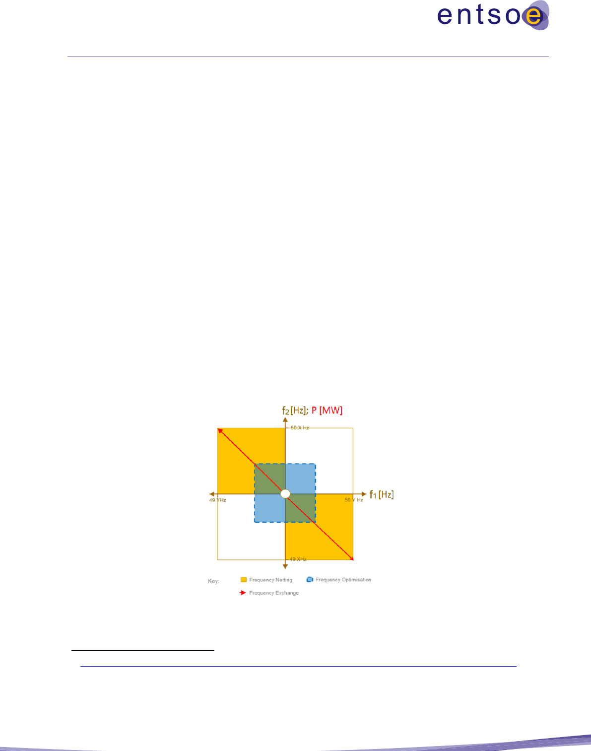
85
5.8.3 B8.2 Frequency Stability (capacity aspect)
This indicator has to be considered a ‘non-mature’ indicator
Introduction
Frequency stability is defined as the ability of a power system to maintain a steady frequency within a
nominal range, following mismatches between generation and demand on a continuous basis or following
a severe system contingency, resulting in a significant imbalance between generation and demand.
Methodology
This section describes the principles behind these types of services, but does not yet put forward a specific
methodology to be applied to arrive at quantitative/monetised results, which require further analysis and
testing. The final methodology should follow in the Implementation Guideline or in a future version of the
CBA Guideline.
Between Synchronous Areas (SAs), i.e. ‘frequency coupling’:
Between Synchronous Areas, frequency support services are officially known as ‘frequency coupling
services’, as described in SOGL. From a legislative perspective, both frequency capacity exchange as well
as frequency capacity sharing are allowed based on Art. 171/172 of SOGL. The allowed technical services,
or products, across HVDC links between SAs are described in the ENTSOE SOC approved paper
46
and
consist of frequency netting (FN), frequency exchange (FE) and frequency optimisation (FO). These are
illustrated in Figure 10:
Figure 10: Illustration of the frequency netting and exchange
46
https://docstore.entsoe.eu/Documents/SOC documents/Operational_limits_and_conditions_for_frequency_coupling-summary_report.pdf

86
The specific limits and conditions to respect are described in the Synchronous Area Operational
Agreements (SA-OA), which inherently cap the maximum potential of any benefits by setting up such
services. The paper is in line with the stipulations set forward in Art. 171/172 of the SOGL. Across HVDC-
cables, such services can indeed be implemented and unlock specific benefits that could theoretically be
monetised (FCR capacity exchange or sharing) or non-monetised (general increase of frequency quality).
Frequency netting & optimisation contribute to the overall frequency quality of both connecting SAs.
These benefits cannot be currently monetised in the CBA methodology as the direct relationship between
frequency quality and the total amount of FCR reserves is not available. Only a qualitative assessment is
possible, or quantification of the frequency quality indices. Frequency exchange requires physical FCR
backup on the providing SA side and hence enables the exchange of FCR capacity, provided the service is
100% available over the HVDC link. Such a setup could theoretically be monetised; however, a proper
methodology cannot yet be proposed.
The benefits of the above-described services can be unlocked by certain grid development projects that
enable additional HVDC links between SAs, provided the considered project has the technical capacity to
enable such services (which should be included in the CAPEX). Pending further analysis and a final
methodology in the Implementation Guideline or the next CBA version, the assessment of those benefits
could work as follows:
For frequency netting and optimisation, in cases where the frequency quality contribution is systematic,
both connecting SAs could agree in a sharing agreement to reduce the overall amount of FCR obligation.
This is provided that the resulting frequency quality remains within the legal limits imposed by SOGL. In
the event this volume could be accurately and realistically estimated, welfare benefits from other markets
(SEW in DA/ID/balancing markets) can be calculated because of a reduced overall FCR obligation.
For frequency capacity exchange, the welfare benefits (SEW in DA/ID/balancing markets) are calculated
by more optimally allocating the overall FCR obligation. As a cautionary note, this assumes that the
allocation can be done in the most optimal manner; however, in practice FCR auction clearing happens
before DA clearing. Therefore, the net effect can also be negative. Frequency exchange gives access to
more (potentially cheaper) resources that can provide FCR.
Within a Synchronous Area:
Within a Synchronous Area, only frequency capacity exchange is allowed (not sharing), as described in
Art. 163/164 of SOGL. Limitations for the capacity exchange (Annex VI of SOGL) stipulate fixed limits
of 30% of initial FCR obligations per LFC block for the CE SA, so theoretically there is no direct link to
any grid development projects there – hence no direct benefits.
However, as described in other SAs (non-CE) or within LFC-areas of the same LFC-block within CE, cases
where internal congestions would be alleviated, or a more even distribution of FCR can be obtained in the
case of network splitting, facilitated by those potential grid development projects, benefits could be present
by giving access to more or cheaper assets that can then deliver the FCR service. This could theoretically
result in a more optimal system operation (reducing overall system/fuel costs). The latter is also described
in Art. 154 §4 of SOGL where geographic limitations could indeed apply that exclude certain units from

87
participating, which would, if resolved by certain grid development projects, then increase the overall
optimality of the system. To calculate or monetise such benefits, very specific localised information should
be available and integrated with other welfare calculations in DA/balancing markets, in order to determine
the effective monetised benefit.
5.8.4 B8.3: Black start services
This indicator has to be seen as ‘non-mature’ indicator
Introduction
This section proposes a methodology for how to assess black start services’ contribution to the SEW of
Europe.
Black start capability means that a power generating facility has the capability of recovering from a total
shutdown through a dedicated auxiliary power source without any electrical energy supply external to the
power-generating facility itself. For a power generating facility to provide black start services, there are
certain criteria that need to be fulfilled, which are described in the connection code Requirements for
Generators.
This type of service is normally contracted or imposed by TSOs to ensure that a minimum level of
generation capacity is available for re-energising the power system after the event of a blackout in the
entire, or part of, the control area. Such services are typically described and required by the network code
on electricity Emergency and Restoration
47
, and national legislation.
Certain grid development projects (internal or cross-border reinforcements) might reduce the need of the
total required volume and/or unlock pathways for contracting more price-efficient units (lower fuel costs).
This potentially reduces the overall system costs and contributes to overall welfare in other markets (e.g.
wholesale or balancing markets) as more, typically peaking, units would consequently become available.
They could also help to avoid new investments costs and reduce the blackout time.
5.8.5 B8.4 Voltage/reactive power services
This indicator has to be considered a ‘non-mature’ indicator
Qualitative description
Voltage or reactive power services/reserves are required from a TSO perspective to satisfy the SOGL
regulation and are also described in national legislation. Typically, these services are contracted or imposed
by TSOs, for a certain minimum level, on specific locations of the grid on existing market flexible units to
ensure the voltage quality remains within the necessary system security limits. Alternatively, these services
can also be ensured by investments in passive elements (capacitors/reactors) or active elements (power
electronic devices such as STATCOMs).
47
https://eur-lex.europa.eu/legal-content/EN/TXT/PDF/?uri=CELEX:32017R2196&from=EN

88
5.9 B9: Reduction of Necessary Reserve for Redispatch Power Plants
Introduction
This benefit indicator can only be calculated when applying redispatch simulations (for a detailed
description on redispatch simulations see section 6.3) for the project assessment and must be added to the
set of benefit indicators as described above.
The redispatch changes the cost-optimal dispatch by exchanging cheaper units for more expensive units.
This leads to situations where more peaking units are more likely to be running. In some countries, the
power plants necessary for providing the maximum redispatch capacity are provided for using specific
contracts.
Therefore, the maximum redispatch power is a direct indication of the need for reserve power plants and
the difference (with and without the project) gives a direct indication of the change in needed reserve power
plants.
Methodology
The capacity of necessary reserves for redispatch (in MW) can be determined by performing the comparison
of the maximum power of redispatch, with and without the project, as received from year-round- redispatch
simulations.
The maximum redispatch power is defined as the maximum of the hourly redispatch power that is calculated
by summing up all redispatch actions within the respective hour.
Indicator definition:
• Definition: Change in needed reserves of redispatch power plants.
• Relevance: The maximum redispatch power is a direct indication of the need for
reserve power plants and the difference (with and without the project) gives a direct
indication of the change in needed reserve power plants.
Indicator calculation:
• Model: Redispatch simulations; based on a redispatch cost comparison with/without
the project.
• Quantitative measure: this indicator is directly given in monetary values.
• Monetisation: per definition monetised and given in €/year
Interlinkage to other CBA indicators:
• B1, B2, B3, B4, B5

89
Note: In principle, this methodology can only be applied for projects located in countries that have a specific
mechanism for contracting redispatch reserve power plants or connecting countries where at least one
country has such a mechanism. If such a mechanism does not exist for the respective countries, an
assumption for the allocation-costs has to be made within the study-specific Implementation Guideline.
Monetisation
The quantification of the benefit is relative to the reduction of the maximum amount of necessary redispatch
in MW and can be monetised using the statistical analysis of the costs of reserve from power plants, i.e.,
from changing capacity constraint payments.
Example: Internal project in country A
A fictitious example of this indicator is provided for an internal project in country A, as follows:
It is assumed that within country A, a mechanism for allocating redispatch power plants exists and that the
assessment has been performed using redispatch simulations. The project is part of the reference grid so the
TOOT method will be applied. The following process steps are adhered to:
1. Calculate the redispatch power with and without the project for each hour of the year
2. Find the maximum redispatch power for both cases (with and without the project):
RD
power
(with) = 16000 MW, which appears in hour 3465
RD
power
(without) = 18000 MW, which appears in hour 5687
3. Build the delta:
RD
power
(delta) = 18000 MW – 16000 MW = 2000 MW
4. Monetise the benefit with 20k€/MW of the allocated redispatch power plant:
B11 = 2000 MW * 20k€/MW = 40 M€
Double-counting:
The risk of double accounting is not given because this benefit indicator can only be applied to projects
located in countries where a specific mechanism for allocating redispatch power plants exists, and in reality
the costs for allocating them must be paid independently if the respective capacity will be used or not.
Furthermore, even when these redispatch reserves are needed payments, the allocation payments and the
actual redispatch costs have to be taken. However, within the simulations, only the latter part is considered,
and the reduction of allocation payments needs to be added to the overall project benefit.

90
Table 15: Reporting Sheet for this Indicator in the TYNDP
Parameter
Source of Calculation
Basic Unit of Measure
Monetary Measure
Level of Coherence of
Monetary Measure
Reduction of necessary
reserves for redispatch
power plants
Redispatch studies
(substitution effect)
MW
€/yr
(market-based)
National

91
5.10 C1: Methodology for CAPital EXpenditure (CAPEX)
Capital expenditure (i.e. CAPEX) is the cost of developing or delivering physical assets.
CAPEX figures are to be declared as real values (i.e. not considering inflation) for each investment. The
values are expressed as constant year-of-study values. For example, for TYNDP 2024 the values are
represented in constant 2024 values.
The capital expense for an investment is to be aggregated and represented as a single value in the year that
it is commissioned. Where a project is comprised of several investments, the aggregated real value of the
expected CAPEX for each investment and the year that the investment is to be commissioned should be
provided.
The terminal values (i.e. the value of the assets at the end of the assessment period) are assumed to be zero.
The costs shall be reported according to the investment status and related uncertainties in the following
manner:
• For mature investments with the status of ‘permitting’ or ‘under construction’, costs should be
reported based on the current data of project promoters, together with a clearly explained
uncertainty range.
48
• For non-mature investments of a ‘planned, but not yet in permitting’ or ‘under consideration’
status, the following is relevant:
1. If detailed project cost information is available, this should be used and the same principle
applied as for mature investments.
2. If detailed project cost information is not usually available, the project promoters will be
required to use standard investment costs, which will be provided by ENTSO-E in the context
of the TYNDP. To account for the specific circumstances and complexities of the project, these
costs are to be multiplied by a clearly defined project-specific complexity factor.
Complexity factors are to be applied in the following manner:
a. To provide a range for the standard costs per group of assets, including a maximum and
minimum value according to its expectations. In this case, the project promoter is required
to provide an explanation (see Table 16).
49
b. In the case where the project promoter chooses complexity factors that exceed the previous
ranges, the choice should be clearly explained. For example, applying complexity factors
to account for different project characteristics, such as terrain, routing, presence of
48
For example, information presented on National Investment Plans.
49
Taken, for example, from the ACER report, with minimum and maximum interquartile.

92
historical landmarks, presence of other infrastructure, population density, special materials
and designs, protected areas, etc. The complexity factor should be unbundled and applied
to the specific cost categories to build up the project cost.
c. In the case of early phase projects, where the project promoter has limited knowledge of
the project investment costs (including the effect of possible project characteristic
impacts), these costs should be equal to the standard investment costs using a complexity
factor equal to 1.0.
50
The methodology used for determining the projects costs, whether based on detailed information
or taken from standard costs, has to be published.
Finally, the investment costs will be one value to which an uncertainty range is applied.
The range of complexity factors to be applied per asset class is shown in Table 16.
Table 16: Table of maximum and minimum Complexity Factors per group of assets
Investment type
Maximum CF
Minimum CF
AC Onshore Overhead Lines (OHL)
1.30
0.50
AC Onshore Cable
1.20
0.70
Subsea Cables
1.10
0.90
AC Substation
1.30
0.60
Transformer
1.30
0.70
HVDC Converter Station
1.20
0.90
In this manner, the provision of the CAPEX expenses enables the project to be compared with other projects
as they can be discounted using common assumptions to the point in time for which the assessment is
needed (the year in which the study is performed). This step is not requested of the promoter.
CAPEX includes both the capital costs incurred at inception during the construction period; and capital
expenditure incurred later in the project life-cycle. Therefore, two indicators, C1a and C1b, which represent
the asset costs at inception and the ongoing asset costs during the original assets’ operation respectively,
represent CAPEX.
C1a: Inception CAPEX
Inception CAPEX is the capital costs incurred at the inception of the project (i.e. during the construction
period). It includes the following cost categories:
• Costs for permits, feasibility studies, design and land acquisition;
50
This information will be updated in future TYNDPs when project promoters have more detail.

93
• Costs for equipment, materials and execution (such as towers, foundations, conductors, substations,
protection and control systems;
• Costs for temporary solutions necessary to realise a project (e.g. a new overhead line required in
an existing route or the installation of a temporary circuit during the construction period); and
• Expected environmental and consenting costs (such as costs to avoid, environmental impacts or
costs compensated under existing legal provisions, cost of planning procedures).
Example: Project X, which is a cluster of investments A, B and C
For each investment, the promoter should provide the aggregated real value (i.e. excluding inflation
rate) of the expected capital expenditure for the investment and the year that the investment is to be
commissioned. This is illustrated by Project X, which is a cluster of three investments: investment A,
investment B and investment C. Investment A is expected to be commissioned in 2022, whereas
investments B and C are expected to be commissioned in 2023 and 2024, respectively.
The assumption for Project X is that capital expenses for each investment are aggregated and
represented as a single value in the year that it is commissioned.
The project promoter should, therefore, provide the information as illustrated in Table 17.
Table 17: Illustration of Capital Expenditure Information to be provided by Project Promoters
Investment
CAPEX
[M€]
Year of
Commission
Investment A
40*
2022
Investment B
10*
2023
Investment C
20*
2024
[Note*: the investment costs are real values in 2020 (for TYNDP 2020–30) terms]

94
C1b: Sustaining CAPEX
Sustaining CAPEX is the capital expenditure incurred during the assessment period that is necessary to
ensure that the functionality of the original assets realised by the inception CAPEX is maintained. This
includes the following:
• Mid-life interventions or significant and scheduled upgrade of assets that are CAPEX in nature are
also to be included in the evaluation. This would include the expected costs for devices that have
to be replaced within the assessment period (consideration of project life-cycle); and
• Dismantling costs at the end of the equipment life-cycle, where relevant, are also to be included in
the CAPEX cost figures.
All costs falling outside the assessment period are not to be considered. This impacts, for example, the
dismantling costs for projects with lifetimes longer than the assessment period.

95
5.11 C2: Methodology for OPerating EXpenditure (OPEX)
OPEX is the ongoing cost of running the investment or project over the assessment period.
OPEX is represented as an annual average cost. It is applied annually from the first year after
commissioning for the duration of the assessment period.
As mentioned in Section 3.2.5, the values are real values and are to be reported as constant year-of-study
values. For example, for the TYNDP 2020 the values are to be represented as constant 2020 values.
The following costs are to be considered as OPEX:
• Expected annual maintenance costs; and
• Expected annual operation costs.
It is required that OPEX is reported per investment.
It is important to highlight that some annual costs can mistakenly be considered as a component of OPEX,
but do not fall into this category, namely:
• System losses, as they are considered in a dedicated indicator.

96
5.12 General Statements on Residual Impacts
The main objective of transmission system planning is to ensure the development of an adequate
transmission system that:
• Enables safe system operation;
• Enables a high level of SoS;
• Contributes to a sustainable energy supply;
• Facilitates grid access for all market participants;
• Contributes to internal market integration, and facilitates competition and harmonisation;
• Contributes to improving the energy efficiency of the system; and
• Enables cross-country transmissions.
The TYNDP highlights the manner in which transmission projects of European Significance contribute to
the EU’s overall sustainability goals, such as CO
2
reduction or the integration of RES. On a local level,
these projects may also impact other EU sustainability objectives, such as the EU Biodiversity Strategy
(COM 2011 244) and landscape protection policies (European Landscape Convention). Moreover, new
infrastructure requires careful implementation though appropriate public participation at different stages of
the project, considering the goals of the Aarhus Convention (1998) and the measures foreseen by the
Regulation (EU) 2022/869.
As a rule, the first measure to deal with the potential negative social and environmental effects of a project
is to avoid causing the impact (e.g. through routing decisions) whenever possible. Steps are also taken to
minimise impacts through mitigation measures, and in some instances compensatory measures, such as the
creation of a wildlife habitat, may be a legal requirement. When project planning is in a sufficiently
advanced stage, the cost of such measures can be estimated accurately, and they are incorporated into the
total project costs (listed under indicator C1).
As it is not always possible to (fully) mitigate certain negative effects, the indicators 'social impact' and
'environmental impact' are used to:
• Indicate where potential impacts have not yet been internalised, i.e. where additional expenditures
may be necessary to avoid, mitigate and/or compensate for impacts, but where these cannot yet be
estimated with sufficient accuracy for the costs to be included in indicator C1; and
• Indicate the residual social and environmental effects of projects, i.e. effects that may not be fully
mitigated in the final project design and cannot be objectively monetised.
Particularly in the early stages of a project, it may be unclear whether certain impacts can, and will,
eventually be mitigated. Such potential impacts are included and labelled as potential impacts. In
subsequent iterations of the TYNDP, they may disappear if they are mitigated or compensated for or lose
the status of potential impact (and become residual) if it becomes clear that the impact will not eventually
be mitigated or compensated for.

97
When insufficient information is available to indicate the (potential) impacts of a project, this will be made
clear in the presentation of project impacts in such a manner that 'no information' cannot be confused with
'no impact'.
In its report on Strategic Environmental Assessment for Power Developments, the International Council on
Large Electric Systems (CIGRÉ, 2011) provides an extensive overview of factors relevant for performing
a Strategic Environmental Assessment (SEA) on transmission systems. Most indicators in this report were
already covered by ENTSO-E's CBA guideline, either implicitly via the additional cost their mitigation
creates for a project or explicitly in the form of a separate indicator (e.g. CO
2
emissions). However, three
aspects (‘biodiversity’, ‘landscape’ and ‘social integration of infrastructure’) could not be quantified clearly
or objectively via an indicator or through monetisation. Previously, these were addressed in the TYNDP by
an expert assessment of the risk of delays to projects, based on the likelihood of protests and objections to
their social and environmental impacts. Particularly for projects in an early stage of development, this
approach improves assessment transparency as it provides a quantitative basis for the indicator score.
To provide a meaningful yet simple and quantifiable measure for these impacts, the new methodology
improves on this indicator by giving an estimate of the number of kilometres required for a new overhead
line (OHL), underground cable (UGC), or submarine cable (SMC) that might have to be located in an area
that is sensitive for its nature or biodiversity (environmental impact) or its landscape or social value (social
impact; for a definition of ‘sensitive’ see below).
When first identifying the need for additional transmission capacity between two areas, one may have a
general idea about the areas that will be connected, whereas more detailed information on, for instance, the
exact route of such an expansion is still lacking as routing decisions are not taken until a later stage. In the
early stages of a project, it is often difficult to determine anything concrete about the social and
environmental consequences of a project, let alone determine the cost of mitigation measures to counter
such effects. Therefore, the quantification of these indicators will be presented in the form of a range, of
which the ‘bandwidth’ tends to decrease as the project progresses in time and information increases. In the
very early stages of development, it is possible that the indicators are left blank in the TYNDP and are only
scored in a successive version of it when some preliminary studies have been conducted and there is at least
some information available to base such scoring upon. A strength of this type of measure is that it can be
applied at a rather early stage of a project when the environmental and social impact of projects is generally
unclear and mitigation measures cannot yet be defined. In subsequent iterations of the TYNDP, as route
planning advances and specification of mitigation measures becomes clearer, the costs will be internalised
in ‘project costs’ (C1) or indicated as ‘residual’ impacts.
As soon as a global idea of the alternative routes that can be used has been determined, a range with
minimum and maximum values for this indicator can be established. These indicators will be presented in
the TYNDP along with the other indicators, as specified in ENTSO-E's CBA Guideline, with a link to
further information. The scores for social and environmental impact will not be presented in the TYNDP
by means of a colour code. These impacts are highly project-specific and it is difficult to express these
completely, objectively and uniformly on the basis of a single indicator. This consideration has led to the
use of ‘number of kilometres’ as a measure to provide information about projects in a uniform manner,
while respecting the complexity of the underlying factors that compose the indicators. Attaching a colour
code purely on the basis of the notion ‘number of kilometres’ would imply that a ‘final verdict’ has been

98
passed regarding the social and environmental sensitivity of the project, which would not be correct because
the number of kilometres that a line crosses through a sensitive area is only one aspect of a project's true
social and environmental impact.
In the case of a replacement project, a residual impact indicator can also attain a zero or negative (i.e. having
a beneficial environmental or social impact) when the affected sensitive area is reduced by the project, i.e.
the ‘number of kilometres’ becomes zero or negative.

99
5.13 S1: Methodology for Residual Environmental Impact
Introduction
Environmental impact characterises the local impact of the project on nature and biodiversity, as assessed
through preliminary studies.
This indicator only considers the residual impact of a project, i.e. the portion of impact not fully accounted
for under C1 and C2. It is expressed in terms of the number of kilometres that an overhead line or
underground/submarine cable may run through environmentally 'sensitive' areas, as defined in 5.16 General
Statements on Residual Impacts.
Methodology
The residual environmental impact is described using the following three descriptors:
• Stage: Refers to the stage of the project or investment. This is important as it gives an indication of
the extent and accuracy at which the environmental impacts can be measured;
• Potential impact: Refers to the assessment of the potential effects that the infrastructure associated
with a project or investment will have on nature and biodiversity.
51
It is measured by the distance
(km) that the infrastructure will be located within an environmentally sensitive area; and
• Type of sensitivity: Defines why this area is considered sensitive.
The assessment of impacts that may qualify an area as environmentally 'sensitive' for the construction of
overhead lines or underground cables, specifically with regard to biodiversity, are addressed by the
following Directives or International Laws:
• Habitats Directive (92/43/EEC);
• Birds Directive (2009/147/EC);
• RAMSAR site;
• IUCN key biodiversity areas;
• Marin Strategy Framework Directive (2008/56/EC); and
• Other nature protection areas under national law.
51
The EC has formulated its headline target for 2020 as: ‘Halting the loss of biodiversity and the degradation of ecosystem services in the EU by
2020, and restoring them in so far as feasible, while stepping up the EU contribution to averting global biodiversity loss.’

100
Example: Assessment of hypothetical investments A, B, C, and D
The residual environmental impact of four hypothetical investments (i.e. A, B, C and D) is illustrated in the
table below:
Table 18: Residual impact examples
Investment
Stage
Impact
(Distance within environmentally
sensitive area) [km]
Sensitivity type
Further information (Link to
be provided)
A
Planned
Yes
(a. 50 to 75 km;
b. 30 to 40 km)
a. Birds
Directive
b. Habitats
Directive
e.g. Big Hill SPA
(www….)
B
Permitting
No
(www….)
C
Planned
Yes
(20 km)
Habitats
Directive
(www….)
D
Under
consideration
N.A
N.A
(www….)
For mature investments in the ‘permitting’ or ‘under construction’ status, the elements listed should be
reported based on the current data of the project promoter, together with the reference to the environmental
impact assessment performed to identify those elements.
For non-mature investments (classified as ‘planned, but not yet in permitting’ and ‘under
consideration’), two cases can be distinguished. If the elements mentioned are available because of an
environmental assessment already performed by the promoter or competent NRA, they should be reported
as in the case of mature investments. In all other cases where an environmental assessment study is not
available or not fit to provide the necessary elements, in the context of the TYNDP, ENTSO-E should
specify (in a dedicated space of the project sheet) that given that the actual route of the project might not
be defined due to the low degree of maturity of its investment(s), an environmental assessment is not yet
available.

101
5.14 S2: Methodology for Residual Social impact
Introduction
Social impact characterises the project impact on the local population, as assessed through preliminary
studies. It is expressed in terms of the number of kilometres that an overhead line or underground/submarine
cable may run through socially sensitive areas, as defined in section 5.16 General Statements on Residual
Impacts. This indicator only takes into account the residual impact of a project, i.e., the portion of impact
that is not fully accounted for under C1 and C2.
Methodology
The residual environmental impact is described using the following three descriptors:
• Stage: Refers to the stage of development of the project or investment. This is important as it gives
an indication of the extent to which social impact can be measured at a particular moment.
• Potential impact: Refers to the assessment of the potential effects that the infrastructure associated
with the project or investment will have on densely populated or protected areas in its proximity.
It is measured by the distance (km) of the infrastructure that is located within socially sensitive
areas.
• Type of sensitivity: Defines why this area is considered to be sensitive.
The following definitions provide an overview of impacts that may qualify an area as socially 'sensitive',
with respect to the construction of an overhead line or underground cable:
Social impact
• Sensitivity regarding population density:
o Land that is close to densely populated areas (as defined by national legislation). As a
general guidance, a dense area is an area where population density is superior to the
national mean.
o Land that is near to schools, day-care centres or similar facilities.
• Sensitivity regarding landscape: protected under the following Directives or International Laws:
o World heritage;
o Land within national parks and areas of outstanding natural beauty;
o Land with cultural significance; and
o Other areas protected by national law.

102
Example: Assessment of hypothetical investments A, B, C, and D
The residual social impact of four hypothetical investments (i.e., A, B, C and D) is illustrated in the table
below:
Table 19: Residual social impact example
Investment
Stage
Impact
(Distance within environmentally
sensitive area) [km]
Sensitivity Type
Further
information
(Link to be
provided)
A
Permitting
Yes (20 to 40 km)
Dense area
(www….)
B
Planned
Yes (100 km)
European Landscape
Convention
(www…)
C
Planned
No
Submarine cable
(www….)
D
Under
construction
Yes (50 km)
Dense area, OHL
(www….)
For mature investments in the ‘permitting’ or ‘under construction’ status, the elements listed should be
reported based on the current data of the project promoter, together with the reference to the social impact
assessment performed to identify those elements.
For non-mature investments (classified as ‘planned, but not yet in permitting’ and as ‘under
consideration’) two cases can be distinguished. If the elements mentioned are available because a social
assessment already been performed by the promoter or competent NRA, they should be reported as in the
case of mature investments. In all other cases, where a social assessment study is not available or not fit to
provide the necessary elements, then ENTSO-E, in the context of the TYNDP, should specify this in a
dedicated space of the project sheet. The note should state that given that the actual route of the project
might not be defined yet because of the low degree of maturity of its investment(s), a residual social impact
assessment is not yet available.

103
5.15 S3: Methodology for Other Residual Impact
The Other Residual Impact (S3) indicator lists the impact(s) of a project that are not covered by indicators
S1 and S2. These impacts may be positive or negative.
Submitting these other impacts is the responsibility of the project promoter and will be included as a list in
the TYNDP assessment results.
Impacts that are accounted for by indicators S1 or S2 should not be included under this indicator.

104
6 Supplemental methodologies
6.1 Contribution to Union Energy Targets (ET)
ET1: Interconnection Targets
The EC established the Expert Group on electricity interconnection targets in March 2016. The Expert
Group's aim was to provide technical advice to the Commission on the extension of the 10% electricity
interconnection target (defined as import capacity over installed generation capacity in an EU country) to
15% by 2030, while considering the costs aspects and the potential of commercial exchanges in the relevant
regions. The Expert Group transmitted its report in October 2017.
The Expert Group recommends that the development of additional interconnections should be considered
if any of the following three thresholds is triggered:
• Minimising price differentials: MS should aim to achieve yearly average of price
differentials as low as possible. The Expert Group recommends €2/MWh between relevant
countries, regions or bidding zones as the indicative threshold to consider developing
additional interconnectors.
• Ensuring that electricity demand, including through imports, can be met in all conditions:
in countries where the nominal transmission capacity of interconnectors is below 30% of
their peak load, options for further interconnectors should be urgently investigated:
nominal transmission capacity / peak load 2030
• Enabling export potential of excess renewable production: in countries where the nominal
transmission capacity of interconnectors is below 30% of their renewable installed
generation capacity, options for further interconnectors should urgently be investigated:
nominal transmission capacity / installed renewable generation capacity 2030
The Expert Group recommends that any project related to interconnection capacity, helping the MS reach
any of the 30% thresholds, must apply for inclusion in the TYNDP and future lists of PCI. In addition,
countries above the 30% but below 60% thresholds in relation to their peak loads and renewable installed
generation capacity are requested to regularly investigate possible options of further interconnectors
regularly. In addition, as a condition sine qua non, each new interconnector must be subject to a
socioeconomic and environmental CBA and implemented only if the potential benefits outweigh the costs.
ET2: Energy Efficiency
According to the EC, Europeans should lower their energy bills by saving energy. By using energy more
efficiently, energy consumption can be reduced. The EC sets energy efficiency targets which translate to
lower primary and final energy consumption. Energy efficiency (EF) can be defined as

105
Thereby, primary energy usage can be regarded as an input to the energy system and is the overall usage of
all primary energy carriers that can be extracted from the market simulations (e.g. methane, hydrogen, etc.).
The final energy consumption is the conventional demand of end-use appliances and can also be extracted
from the market simulations. Any variation in energy efficiency unlocked by a project
contributes to the overall European target and can be reported in the study-specific project sheets.
ET3: Renewable Penetration
The share of energy from renewable sources shall be calculated as the gross final consumption of energy
from renewable sources divided by the gross final consumption of energy from all energy sources,
expressed as a percentage
52
.
The numerator, ‘gross final consumption of electricity from renewable energy sources’, shall be calculated
as the quantity of electricity produced in a MS from renewable energy, and the denominator ‘gross final
consumption of electricity’ is, for the purpose of the calculations defined as the generation from all energy
sources. For both numerator and denominator, a detailed overview of generation sources considered have
to be defined within the respective study-specific implementation guidelines.
The evaluation of a project’s impact on the renewable penetration ET3 will then be calculated as a delta
comparison of the RES penetration with and without the project
and can be reported in the study-specific project sheets.
6.2 Methodology for the assessment of Hybrid Projects
6.2.1 Context
Following the ongoing European decarbonisation targets and related EU legislation initiatives (Green
Deal and FIT for 55 legislative package), a massive uptake in offshore RES (predominantly offshore
wind technology) is expected now and in the upcoming decades, aiming at above 60 GW offshore
wind + 1 GW ocean energy by 2030 and 300 GW offshore wind and 40 GW ocean energy by 2050
in European waters, following the EC’s offshore RES strategy.
52
Directive 2009/28/EC of the European Parliament and of the council of 23 April 2009 on the promotion of the use of energy from renewable
sources and amending and subsequently repealing Directives 2001/77/EC and 2003/30/EC

106
Historically, mostly radial connections to onshore bidding zones were developed near-shore,
especially for offshore RES (short distances, AC-technology). For the near future, to fully exploit the
energy potential of the European sea basins, far-out connections will be further exploited. A new set
of technical setups will allow the interconnection-function between bidding zones (on- or offshore)
to be combined with a facilitation of direct wind infeed (RES-connection). For these new
configurations, which are defined below as (offshore) hybrid projects or dual/ multi-purpose
interconnections, additional clarifications are necessary for proper CBA calculations to be performed
in the framework of the European TYNDP.
6.2.2 Hybrid interconnector definition
The hybrid interconnector projects serve at least dual purposes within the electricity sector and
constitutes a new project category related to CBA assessment, which project promoters need to
indicate & provide correct parameters for to facilitate appropriate CBA calculation (see separate CBA
section further). A further development of ‘dual purpose’ is ‘multi-purpose’ in cases the project
integrates other sectors as well (e.g. via electrolysers). This multi-purpose project category, where
other sectors are coupled, is not considered in this document.
The hybrid interconnection setup and dual purpose (see Figure 11) can be defined as a project which
enables an interconnector function between bidding zones (either onshore or offshore) while
simultaneously facilitating a client connection with a certain technology (RES or non-RES;
generation, load or storage; AC (e.g. Kriegers Flak) or DC (e.g. North Sea Windpower Hub)).
Hybrid interconnection projects are mainly expected offshore and are linked to the European Offshore
RES strategy but, in theory, onshore cases could also exist: for instance, a wind farm in a mountain
area with just 1 XB-interconnection (tie-line) passing by to which it could connect, rather than directly
within the onshore bidding zones.
From the perspective of the client, for example an offshore wind project, the client connection will
directly feed in or take off power off an otherwise direct cross-border interconnection (XB-IC) or tie-
line/cable that connects MS bidding zones (BZs).
Based on how a hybrid interconnection setup is developed, two CBA options can be defined, as
defined exhaustively in chapter 3.
• CBA Option 1 expansion of an existing radial client connection through the inclusion of an
XB interconnection (IC)
• CBA Option 2 – project developed anew as a hybrid interconnector
The hybrid interconnection projects target the effective creation of a link between two or more BZs –
meaning the project scope goes beyond anything that remains within one and the same BZ. General
clustering rules should apply to effectively considering the multiple links & OWF(s) connections
together in one project or whether multiple projects need to be created. Once more offshore hybrid
interconnection projects are combined, they effectively result in a multi-terminal or offshore network
setup.
The different project options that can be pursued by project promoters are listed in Figure 11 below,
illustrating the cases for offshore development only – whereas the concepts can also apply onshore.
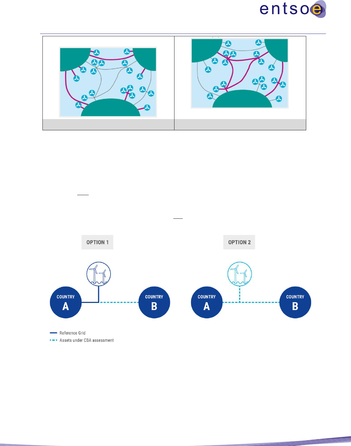
107
Single purpose
Dual purpose (= Hybrid)
Figure 11: figure taken from ENTSO-E Position on Offshore Development–- Summary of Recommendations, July 2021
6.2.3 Hybrid interconnection CBA configuration
Two CBA setups are possible for CBA analysis and are defined as CBA option 1 and option 2 in the
remaining text:
• Option 1: the project is built on top of an already existing or planned radial connected RES by
enabling only an additional interconnector function (which consequently will then also host the
existing or planned RES infeed from the initial radial connection)
• Option 2: the project enables both the RES-integration function (i.e. additional OWF capacity is
integrated into the system through the project) and the additional interconnector function; and the
project is developed anew as a hybrid interconnector
Figure 12: Hybrid CBA fundamental options
For illustration purposes, only the offshore wind technology setup will be illustrated. More complex
variants, where multiple links are built to the same OWF or where meshing is introduced (either
within same market or between BZs), can follow the same logic.
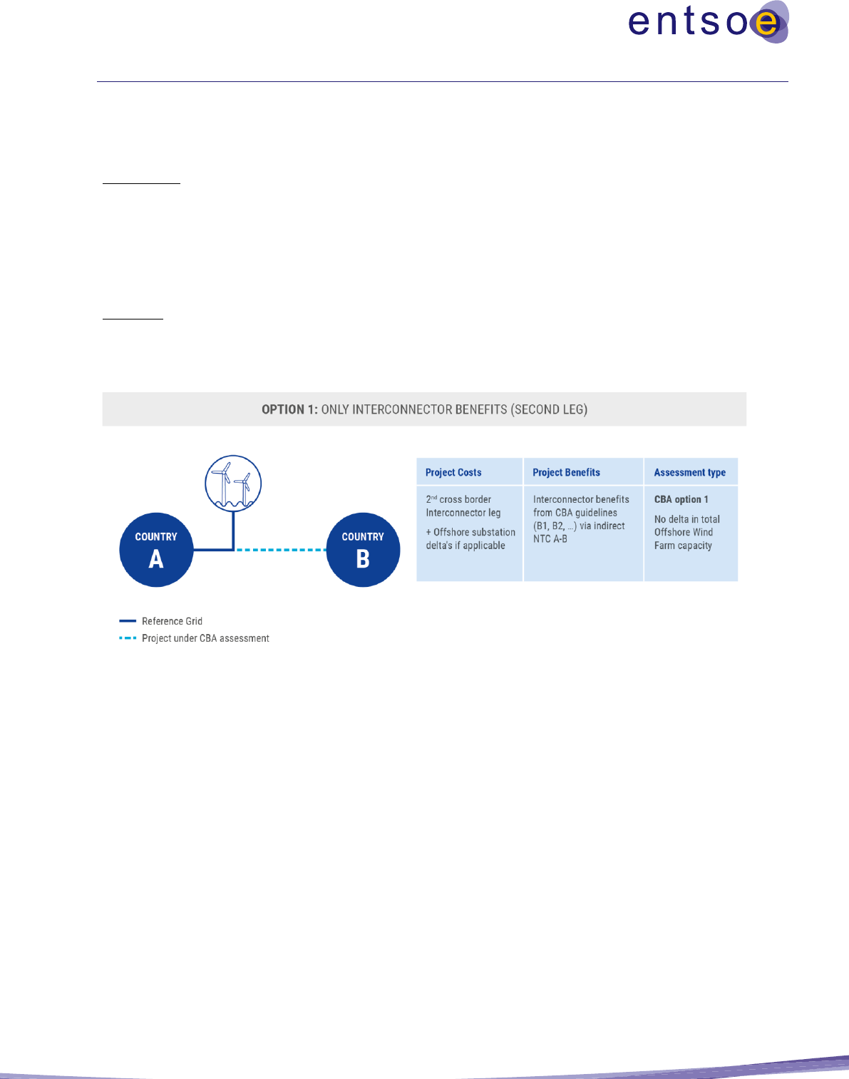
108
6.2.3.1 CBA Option 1
The project transforms the original client connection towards a cross-border (XB) line, by integrating
the offshore RES through building the remaining leg to enable the XB function.
The benefits of market integration (relevant B1, B2, B4, B6 indicators) are enabled by increasing the
transfer capacity between country A and B, as shown in Figure 13, enabled either in a home market
(HM) setup or offshore bidding zone (OBZ) setup. In the case of a home market setup, RES is strictly
allocated to either country A or B, and the created single NTC would be lower compared to the case
of a direct connection between A and B without RES as the offshore RES energy will impact the
options for remaining trade and congest the direct connection.
The costs (CAPEX) scope is defined as the asset of the 2
nd
leg and potential deltas of the targeted
client connection.
CBA option 1 can be summarised in Figure 13 below.
Figure 13: Project cost & benefit scope under CBA Option 1 assessment
6.2.3.2 CBA Option 2
The project builds the necessary leg(s) and simultaneously enables additional RES onto the resulting
link, thereby enabling the dual function together i.e. the interconnection function and RES integration
function. There are principally three different setups possible for CBA option 2:
(1) Either both legs + access for the RES constitute the project entirely, which builds all anew.
(2) Or, in the event a first leg with a radial RES connection is already planned, where on top of now
a hybrid interconnection project will be added. The hybrid interconnection project scope itself for
CBA assessment is then only constituted by the second leg and, crucially, also by additional RES
facilitation on top of the initial radial RES amount. If the radial RES connection is not in the
reference grid, then a sequential CBA assessment is required using both projects.
(3) A radial RES connection is built on a planned or existing XB line, effectively yielding the same
outcome i.e. a hybrid interconnector.
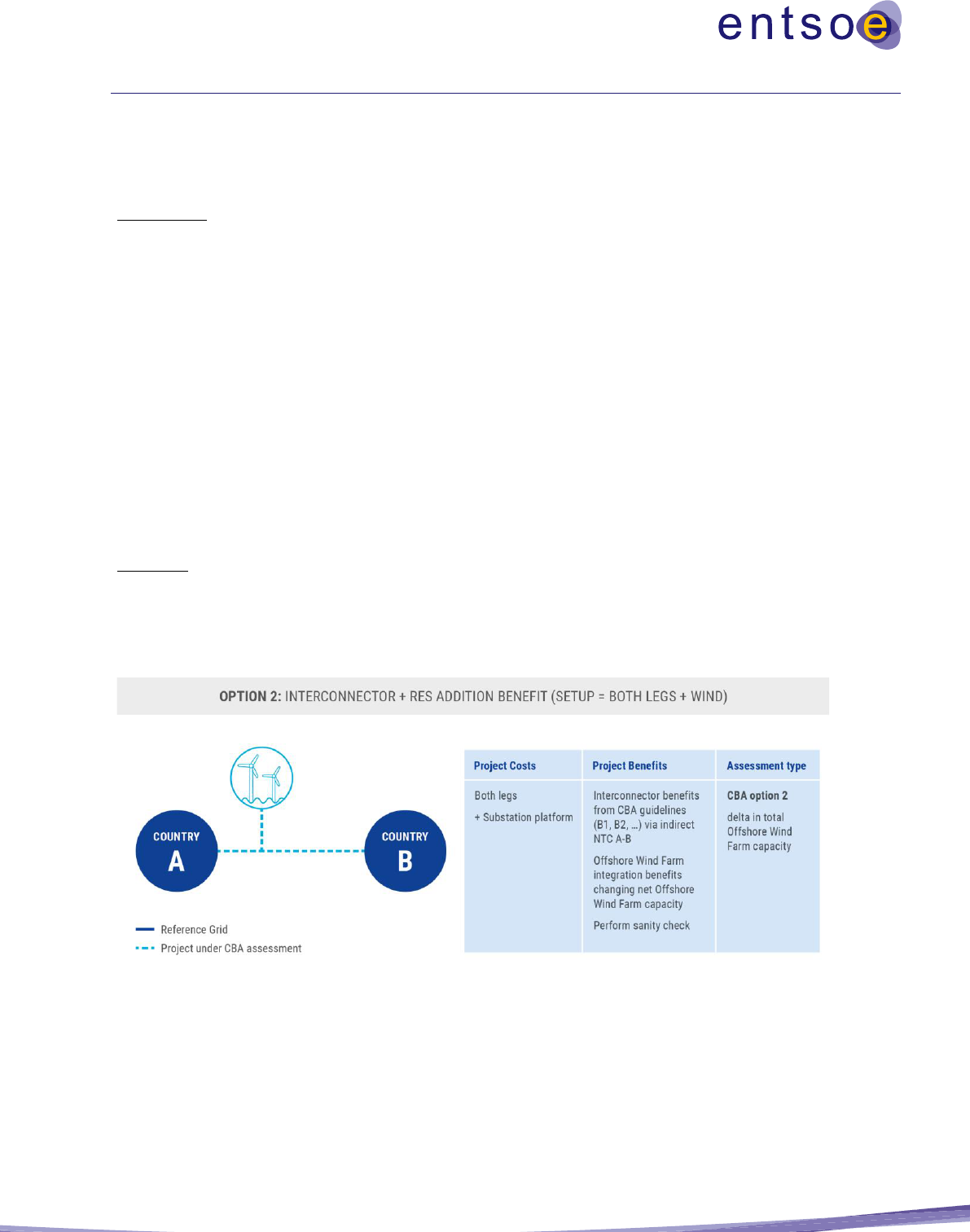
109
For the benefits and costs for setups 1/2/3, it should be acknowledged that between 1 and 2 there is
only the difference in project cost scope, whereas for theoretical case 3 only RES-integration benefits
would be present (with an impact on the remaining NTC between bidding zone A and B dependent
on the chosen market setup HM or OBZ). For the remainder of the text, only setup 1 is illustrated.
The benefits of market integration (relevant B1, B2, B3, B4, B6 indicators) are enabled through the
creation of:
• A single NTC between A and B enabled in a home market setup (1 reduced NTC in total) and the
creation of direct RES integration.
• Double NTC (2 NTCs in total i.e. 1 between country A and RES, and 1 between country B and
RES) enabled in an OBZ setup and the creation of direct RES integration itself.
• The producer surplus of the targeted RES itself needs to be removed from the EU–SEW as a
proxy to warrant the required RES investment. The producer surplus can be calculated as the
dispatched RES feed-in volume for all hours of the considered year, multiplied by the price the
OWF gets, which is determined by the bidding zone in which it is considered. This calculation
can be done ex-post and, in the event the RES is connected to 2 or more bidding zones onshore
in a separate bidding zone setup, it will get the lowest price of all bidding zones to which it is
linked.
• To consider the benefits of RES integration, a sanity check needs to be applied. This sanity check
will be described in the study-specific Implementation Guidelines.
The costs (CAPEX) scope is defined as all legs part of the project scope required to enable the
interconnection function and related substation to enable the RES infeed onto the interconnector (e.g.
offshore this is typically a platform). The costs of the RES asset itself are excluded.
CBA option 2 is summarised in Figure 14 below.
Figure 14: Project cost and benefit scope under CBA Option 2 assessment
The choice between CBA option 1 vs option 2 is up to the project promoter. However, the impact of
the choice should be clear; for example, the consequences for the cost scope of the project (& related
benefits), the implicit inclusion of the scope of the RES project and the need to respect the general
CBA clustering rules when specifying a project and/or requesting a sequential CBA.

110
Additional information to justify the choice must be given by the project promoter.
6.2.4 Radial projects:
To harmonise the methodology for hybrid and radial projects, the CBA option 2 approach could be
applied to radial projects. The assessment of a radial project will consider only the RES integration
benefits (no trade benefits).
The producer surplus of the targeted RES itself needs to be removed from the SEW, as a proxy to
warrant the required RES investment. As for hybrid projects, to consider the benefits of RES
integration, a sanity check needs to be applied. This sanity check will be described in the study-
specific Implementation Guidelines.
The costs scope for radial projects only include the grid connection (cables and platforms); the RES
assets themselves are excluded. This means, for example, for an offshore radial project, that the costs
scope includes only the societal transmission grid assets but not the offshore inter array cables or the
offshore wind farm itself.
6.2.5 NTCs
NTCs should respect the guidance, and hence can be different from the thermal capacity of the
respective legs of the hybrid setup in general and clearly also when different leg sizing is applicable.
NTCs should reflect the HM or OBZ setup chosen, which mainly affects dispatch results in case of
negative price occurrence in one or more bidding zones. As explained for both CBA option 1 and 2,
for the HM setup a reduced NTC concept is to be applied, whereas for the OBZ setup separate
traditional NTCs can be utilised.
The power rating of the different legs and the targeted voltage level are needed and need to be
modelled to most accurately assess, among others, the B5 indicator (grid losses & related
monetization).
6.3 Redispatch simulations for project assessment
Assessing projects by only focusing on the impact of transfer capacities across certain international borders
can lead to an underestimation of the project-specific benefits. This is because most projects also show
significant positive benefits that cannot be covered by only increasing the capacities of a certain border, i.e.
the reduction of internal congestions. This effect is strongest, but not limited to, internal projects that do
not necessarily aim to increase the capacities across specific borders and, therefore, this makes it difficult,
or even impossible, to solely assess them using market simulations.

111
According to the CBA, both internal and cross-border projects can be of pan-European relevance; however,
they all develop GTC over a certain boundary (and sometimes several boundaries), which may or not be an
international border.
Furthermore, as cross-border projects can also have an impact on internal congestions and on the redispatch,
just as internal projects can have an impact on cross-border transfer capacities, the application of redispatch
simulations also needs to be allowed for interconnectors whenever necessary.
The detailed description of the respective methodology is described below.
Generally, to perform the project assessment using redispatch simulations, the following simulation steps
need to be performed:
• Simulation step 1: Perform market simulations to determine the cost-optimal power plant dispatch;
• Simulation step 2: Perform load-flow simulations based on the outcome from step 1 to determine
the line loadings in the observed grid; and
• Simulation step 3: Perform redispatch simulations to identify opportunities to mitigate possible
congestions
53
as achieved from step 2 by redispatching the initial power plant dispatch (taken from
step 1).
These steps might be performed using a single tool or a combination of different tools, but none of them
must be neglected.
Benefit calculation using redispatch simulations
To perform the redispatch simulations, the same delta approach used for market simulations can also be
applied, i.e. the benefits are calculated using TOOT or PINT and multiple TOOT or PINT. The indicators
that can be calculated using redispatch simulations are those defined under the respective indicator.
Following this, the same indicators as for market simulations can be achieved using the redispatch
simulations, i.e. B1, B2, B3, B4. by assessing the impact on the amount of redispatch to eliminate internal
congestions with and without the project.
The redispatch simulations must be aligned with the market studies conducted using the respective
scenarios. To meet this requirement, the market study results (e.g. hourly generation of the specific unit
types) and market study inputs (e.g. capacities of generation types) must be used as an input for the
redispatch assessment. This should include the same main input data-set used for market simulations, which
is summarised below:
• Price assumptions (fuel prices, CO
2
price, and the marginal costs of thermal generation types
calculated from these);
53
The check for whether the congestions have been mitigated by the redispatch needs to be achieved using load-flow simulations

112
• Net-generating capacities for thermal generation types, RES (wind and solar), other RES, other
non-RES and hydro categories (incl. pumping capacities);
• Must-run values of thermal generation types;
• Availability of generating units;
• DSR capacities;
• Demand time series; and
• Fixed exchanges with non-modelled countries.
The main datasets to be used from the market simulation results are as follows:
• Utilisation (hourly time-series) of thermal generation types, DSR and hydro categories (turbining
and pumping);
• Dumped energy time series (on wind, solar, Other RES and Other non-RES generation categories
combined);
• Hourly marginal costs on market nodes; and
• ENS (energy not served) time series.
There are a number of requirements for the grid or network simulations: The simulations should ideally be
based on AC load flows. If this is not possible, or in order to reduce the simulation time to an accepted
level, DC load-flows can be applied. The simulations should be made on a year-round basis. If this is not
possible, representative points in time can be used, as is the case for the losses calculation. The method of
mapping the market simulation results to the grid model (i.e. the distribution of market node level results
to nodal level in the grid model) is to be defined in the Implementation Guidelines and must be consistent
with other grid studies (e.g. the NTC, losses calculations).
Any thermal overloads identified from the network simulations could potentially be mitigated by employing
redispatch simulations. The redispatch simulations should observe the following requirements:
• The balance of the system must be kept (i.e. the rise in generation must be covered by the same
amount of reduced generation);
• The network, or at least pre-defined critical branches, must be free of congestion after the
redispatch is implemented; and
• The redispatch must be implemented in a cost-optimal manner.
The perimeter of the redispatch simulations needs to be defined, and can be defined as follows:

113
• The perimeter should be chosen to cover the grid area influenced by the project. The decision
depends on whether the project is internal or cross-border. For internal projects, the perimeter for
internal projects without significant cross-border impact is typically the country that includes the
project. For cross-border projects, the perimeter is typically the two countries that include the
project on their common border.
• In cases where only part of the country (or countries) is influenced by the project, it is possible to
reduce the perimeter to that part alone, on condition that the reduced perimeter includes all grid
elements relevant for the redispatch analysis. The ‘relevance’ has to be clearly stated and reported.
• In cases where other surrounding countries are also supposed to be significantly influenced by the
project, the perimeter should be extended to include those countries.
Optimisation measures are implemented according to a particular order. The order
54
(or sequence) that is to
be applied and adhered to is as follows:
1. Apply operational measures (e.g. PST, HVDC);
2. Apply the pre-defined set of topological curative actions for each N-1 (or appropriate security
criterion);
3. Optimise thermal power plants based on the dispatch costs of each generator;
4. Optimise storage devices (e.g. hydro generators, batteries, P2G, etc.);
5. Optimise RES;
6. Optimise cross-border power plants and cross-border HVDC links (depending on the perimeter);
and
7. Address the overloading of transmission equipment.
As there are different project types, with different objectives, the simulation methods can also be different,
depending on the objective. Although the objective of cross-border projects may be to increase the capacity
between different countries and market areas, the objective of an internal project may not be to impact
cross-border capacity. Therefore, it would make only little sense to assess these types of projects by
comparing the two different market simulation runs.
To account for different project types, there are two options for applying redispatch simulations:
The first option only uses redispatch simulations
55
to calculate the benefits, whereas the second option
integrates both market and redispatch modelling. The decision regarding which methodology to apply
54
No country-specific differences to this approach have yet been identified. If these are identified, they must be considered.
55
The basis for the redispatch simulation under this option also relies on market simulations. In this case, the project has no NTC impact,
therefore, only the reference market simulation output is used as an input. The different amounts of redispatch needed with and without the
project (in the grid model) make the basis of the assessment.
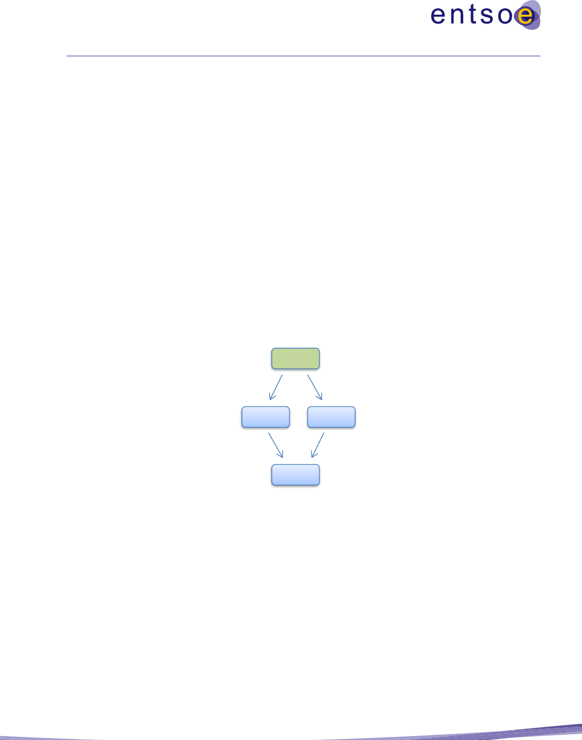
114
depends on the case being assessed. In general, when assessing the market benefits of a project where the
main aim of the project relies on a cross-border level, pure market simulations should be used. For projects
where the main focus is on healing internal congestions, pure redispatch simulations should be used. Of
course, there are also projects that are built to fulfil both needs. Therefore, to cover the full spectrum of
benefits for different types of projects, a variation in methodologies or a combination of methodologies
should be used. The choice of which method to use is for the project promoter to decide. However, the
chosen method needs to be displayed with a justification of the respective choice. In cases where the
assessment uses a combination of market and redispatch studies, the benefits must be displayed separately
for market and redispatch studies.
Note:
The following options are only related to the benefit calculation itself; to perform redispatch simulations,
preceding market and network simulations are always necessary.
Option 1: Calculation of benefits using pure redispatch:
The benefits for projects with a focus mainly on internal impacts can solely be assessed by using redispatch
simulations. Using a single market simulation output, two different redispatch simulations (i.e. one with the
project and the other without the project) need to be performed (TOOT/PINT). The process needs to respect
the conditions described above, and is illustrated below:
Where:
MS1 refers to market simulation reference NTCs;
RD1 refers to the redispatch run with reference network;
RD2 refers to the redispatch run, with the project being assessed taken out/in (TOOT/PINT); and
∆RD refers to the difference between RD1 and RD2 unit commitment (different generation costs,
different CO
2
outputs, etc.)
RD1
RD2
MS1
∆RD
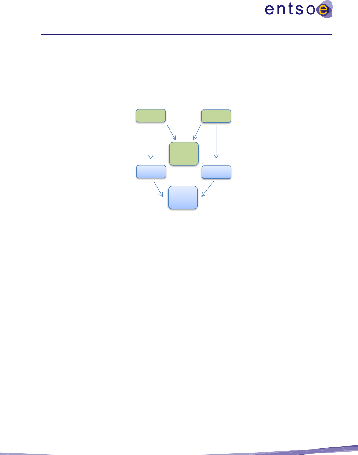
115
Option 2: Calculation of benefits using a combination of border-NTC-variation and redispatch:
The benefits of some projects mainly depend on internal bottlenecks, but can also have significant cross-
border impact. In this case, a two-step approach can be used by combining the assessment using market
simulations with redispatch simulations, with the final result being the sum of both. The process is
illustrated below:
Where:
MS1 refers to the market simulation with reference network;
MS2 refers to the market simulation with the project being assessed taken out/in (TOOT/PINT);
∆MS refers to the difference between MS1 and MS2 unit commitment;
RD1 refers to the redispatch run with reference network;
RD2 refers to the redispatch run with the project being assessed taken out/in (TOOT/PINT);
∆RD refers to the difference between RD1 and RD2 unit commitment; and
∆TOTAL is given by the sum of ∆RD and ∆MS.
The application of redispatch enables the identification of a specific benefit indicator, B9: Reduction of
Necessary Reserve for Redispatch Power Plants, which is discussed in section 5.9.
RD1
MS1
RD2
MS2
SEW
∆RD
SEW
∆MS

116
6.4 Value of Lost Load
VOLL is a measure of the costs for consumers associated with unserved energy (i.e. the energy that would
have been supplied if there had been no outage), and is generally measured in €/kWh. It reflects the mean
value of an outage per kWh (long interruptions) or kW (voltage dips, short interruptions), appropriately
weighted to yield a composite value for the overall sector or nation considered. It is an externality as there
is presently no market for SoS.
The value for VOLL used in project assessments should reflect the real cost of outages for system users,
thereby providing an accurate basis for investment decisions. A level of VOLL that is too high would lead
to over-investment, and a value that is too low would lead to under-investment. Under-investment would
result in an inadequate SoS because the costs of measures to prevent an outage are erroneously weighed
against the value of preventing the outage. The optimal level should correspond to the consumer’s
willingness to pay for SoS. Considering VOLL in project assessments requires that the right balance is
struck between transmission reinforcements (which have a cost, reflected in tariffs) and outage costs.
Transmission reinforcements generally contribute to improving the security and quality of the electricity
supply, reduce the probability and severity of outages, and thereby reduce costs for consumers.
Experience has demonstrated that estimated values for VOLL vary significantly depending on geographic
factors, differences in the nature of load composition, the type of consumers that are affected and their level
of dependency on electricity, differences in reliability standards, the time of year, and the duration of the
outage. Using a general and uniform estimation for VOLL would lead to inconsistency and less
transparency and would greatly increase uncertainties compared to presenting the physical units.
Providing a reliable figure for VOLL, which reflects the actual societal costs of an outage, is vital for a
proper project assessment with a monetised EENS component. When EENS is monetised, this is likely to
shift the focus during interpretation of results away from the underlying values (i.e. a value in MWh that is
different in each hour and in each price zone) because the monetised value is simply included in the
summation of all monetised benefits and costs (e.g. to obtain a simple benefit–cost ratio). This is not
problematic if an appropriate set of VOLL-values exists, which properly consider the spatial, temporal and
actual characteristics associated with the cost of EENS. However, if the values used for VOLL in different
situations are based on disparate calculation methodologies, which is the case under the present state of
knowledge regarding economic valuation of outages, the credibility of the otherwise uniform and
standardised project assessment results is undermined. ENTSO-E, therefore, considers the availability of a
computation methodology that is approved by ACER and the EC as a prerequisite for reporting monetised
values of EENS.
Note that in the absence of a uniform and standardised methodology to compute values for VOLL, EENS
can nonetheless be monetised by stakeholders that make use of CBA results (e.g. the EC during the PCI
process). The energy figure expressed in MWh, which ENTSO-E provides as the SoS indicator in the CBA
evaluation for each project, allows all interested parties to derive a monetised value by using the preferred
VOLL available. In any case, the VOLL values used in the assessment need to be transparently displayed
within the study-specific Implementation Guidelines.

117
6.5 Climate adaptation measures
Project promoters will be asked to state which climate adaptation measures have been taken by the project.
Climate adaptation measures are defined as ‘a process that ensures that resilience to the potential adverse
impacts of climate change of energy infrastructure is achieved through a climate vulnerability and risk
assessment, including through relevant adaptation measures.’ in regulation (EU) 2022/869.
Climate adaptation measures would include all adaptations to an investment to cope with possible
(predicted) future extreme weather events due to climate change. This could include e.g. flooding, extreme
heat or extreme cold, hurricanes, thunderstorms etc.

118
End note.
System development tools are continuingly evolving, and it is the intention that this document will be
reviewed periodically pursuant to Regulation (EU) 2022/869, Art.11 §13 and in line with prudent planning
practices and further editions of the ENTSO-E’s TYNDP document.

119
ANNEXES
I. Generation cost approach
The economic benefit is calculated from the reduction in total generation costs associated with the NTC
variation created by the project. There are three aspects to this benefit:
a. By reducing network bottlenecks that restrict the access of generation to the full European market,
a project can reduce the costs of generation restrictions, both within and between bidding areas.
b. A project can contribute to reduced costs by providing a direct system connection to new, relatively
low cost, generation. In the case of connection of renewables, this is also expressed by benefit B3,
RES Integration.
c. A project can also facilitate increased competition between generators, reducing the price of
electricity to final consumers. The methods do not consider market power, and consequently the
expression of socioeconomic welfare is the reduction in generation costs.
An economic optimisation is undertaken to determine the optimal dispatch cost of generation, with and
without the project. The benefit for each case is calculated from the following relationship:
Benefit (for each time step) = sum of Generation costs without the project (sum over all time steps)
over all sectors – sum of Generation costs with the project (sum over all time steps) over all sectors
The socioeconomic welfare, in terms of savings in total generation costs, can be calculated for internal
constraints by redispatch (see Chapter 2.3 Cross-border versus internal . In any case, the method used for
the SEW calculation must be clearly highlighted.
The total benefit for the horizon is calculated by summarising the benefit for all the hours of the year, which
is done through market studies.

120
II. Total surplus approach
The global socioeconomic welfare is defined as the sum of the total surpluses stemming from the involved
sectors. The total surplus approach takes the value of serving a particular unit of load into account. An
economic optimisation is undertaken to determine the total sum of the producer surplus (difference between
electricity price and generation cost), the consumer surplus (difference between willingness-to-pay the
value of electricity and electricity price for a demand block), the change in congestion rent (difference in
electricity prices between price zones), and possibly the change in cross-sector rent with and without the
project. The total surplus of a specific sector is:
Total surplus = Producer Surplus + Consumer Surplus + Congestion Rents + Cross-Sector Rents
The economic benefit is calculated by adding the producer surplus (a measure of producer welfare), the
consumer surplus (a measure of consumer welfare), the congestion rents for all price areas, as shown in
Figure 16, and possibly the cross-sector rents. The total surplus approach consists of the following three
items:
a. By reducing network bottlenecks, the total generation cost will be economically optimised. This
is reflected in the sum of the producer surpluses, which is defined as the difference between the
prices the producers are willing to supply electricity and the generation costs.
b. By reducing network bottlenecks that restrict the access of import from low-price areas, the total
consumption cost will be decreased. This is reflected in the sum of the consumer surpluses, which
is defined as the difference between the prices the consumers are willing to pay for electricity and
the market price.
c. Reducing network bottlenecks will lead to a change in total congestion rent for the TSOs.
.
A project with an NTC variation between two bidding areas with a price difference will allow generators
in the low-price bidding area to supply load in the high price bidding area. In a perfect market, the market
price is determined at the intersection of the demand and supply curves.
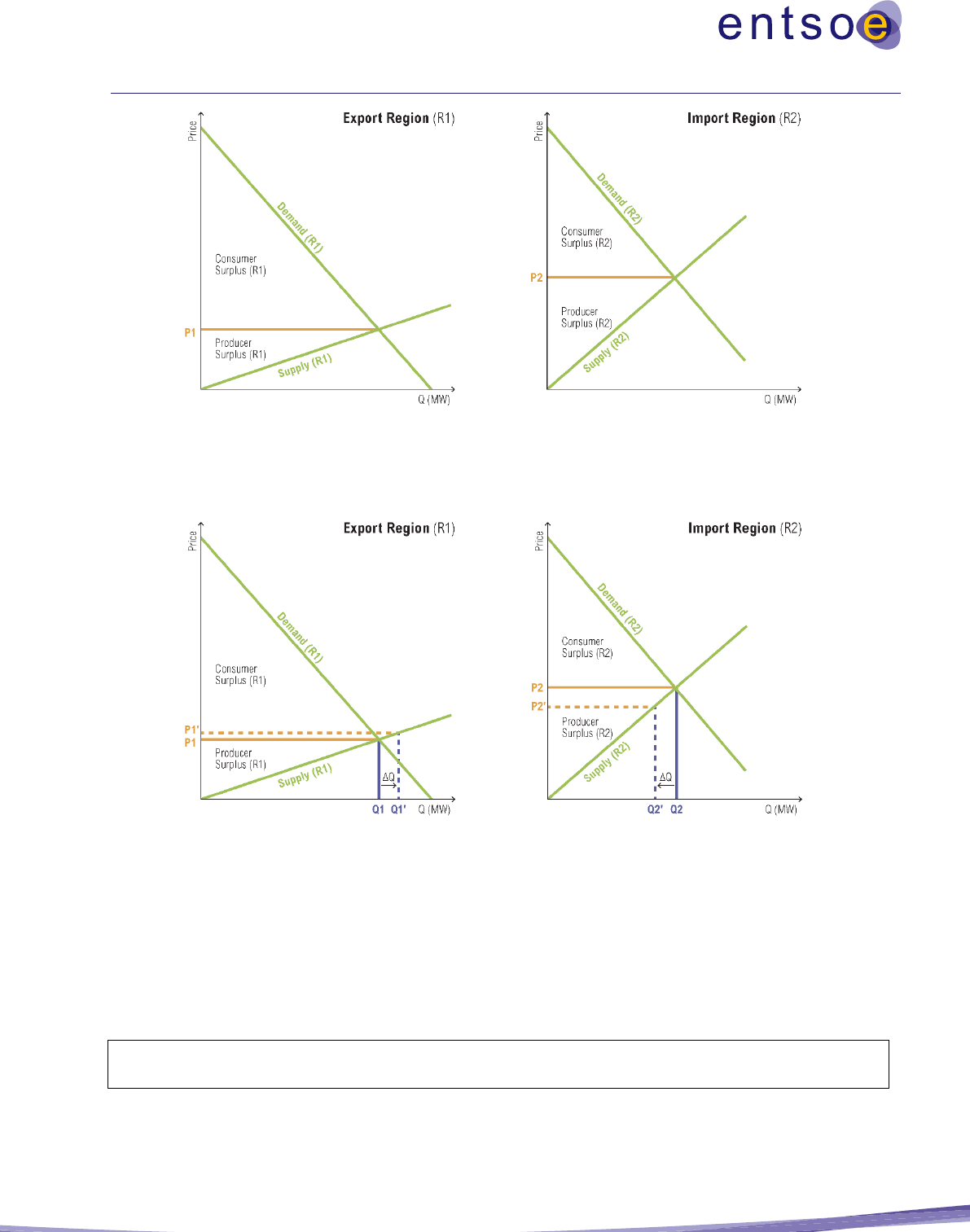
121
Figure 15: Example of an export region (left) and an import region (right) with no (or congested) interconnection capacity
(elastic demand)
Figure 16: Example of an export region and an import region, with a new project increasing the GTC between the two regions
(elastic demand)
A new project will change the price of both bidding areas. This will lead to a change in consumer and
producer surplus in both the export and import areas. Furthermore, the TSO revenues will reflect the change
in total congestion rents on all links between the export and import areas. The benefit of the project can be
measured through the change in socioeconomic welfare. The change in welfare of a specific sector is
calculated by:
Change in welfare = change in consumer surplus + change in producer surplus + change in total
congestion rents + change of cross-sector rents
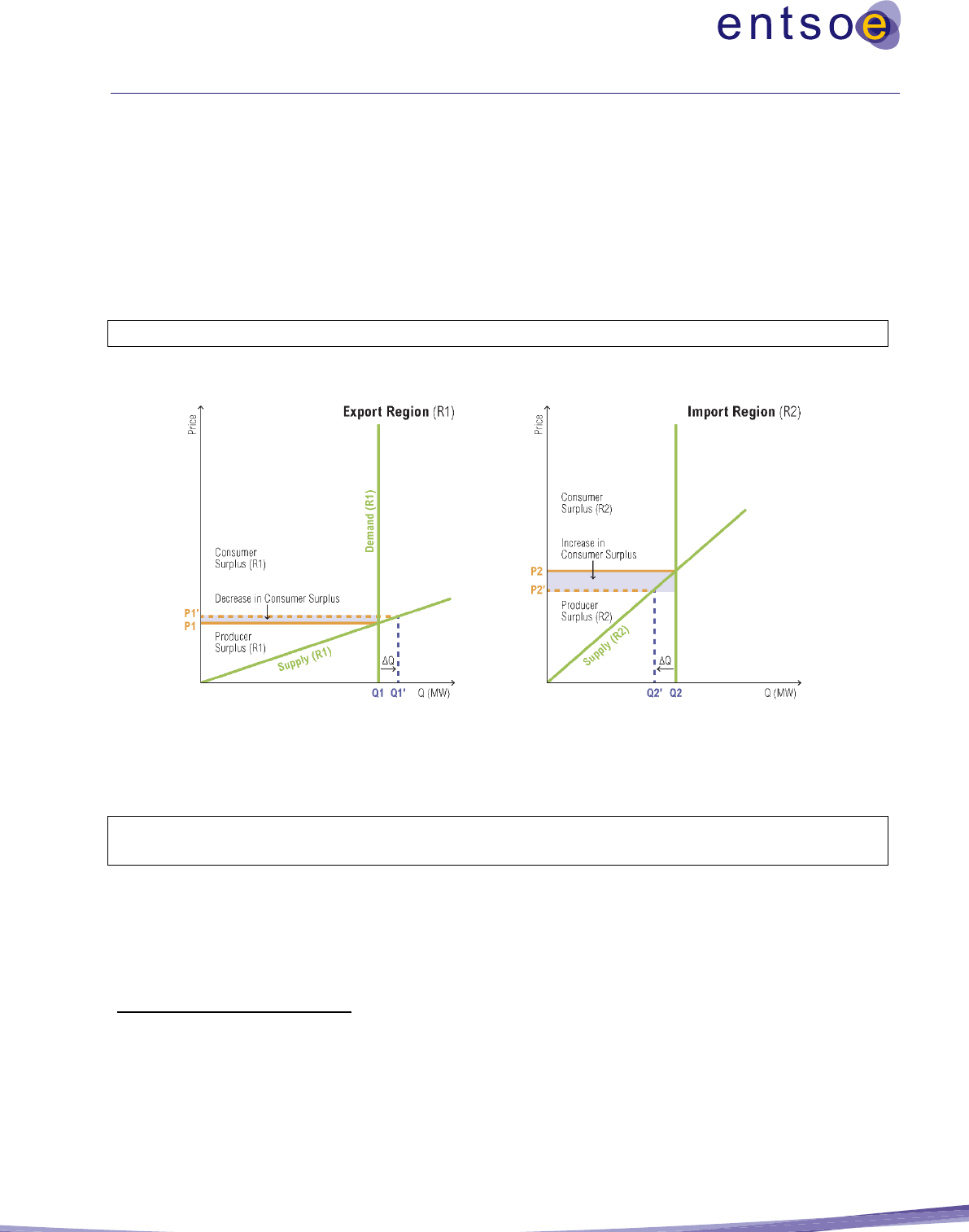
122
The total benefit for the horizon is calculated by summing the benefit for all time steps considered in that
year.
The total surplus is maximised when the market price is at the intersection of the demand and supply curves.
Inelasticity of demand
In the case of the electricity market, short-term demand can be considered as inelastic as customers do not
respond directly to real-time market prices (no willingness-to-pay-value is available). The change in
consumer surplus
56
of a specific sector can be calculated as follows:
For inelastic demand: change in consumer surplus = change in prices multiplied by demand
Figure 17: Change in consumer surplus
The change in producer surplus of a specific sector can be calculated as follows:
Change in producer surplus = change in generation revenues
57
– change in marginal generation
costs
56
When demand is considered as inelastic, the consumer surplus cannot be calculated in an absolute way (it is infinite). However, the variation in
consumer surplus, as a result of the new project, can be calculated nonetheless. It equals the sum for every hour of the year of: (marginal cost of
the area x total consumption of the area)
with the project
– marginal cost of the area x total consumption of the area)
without the project
57
Generation revenues equal: (marginal cost of the area x total production of the area).
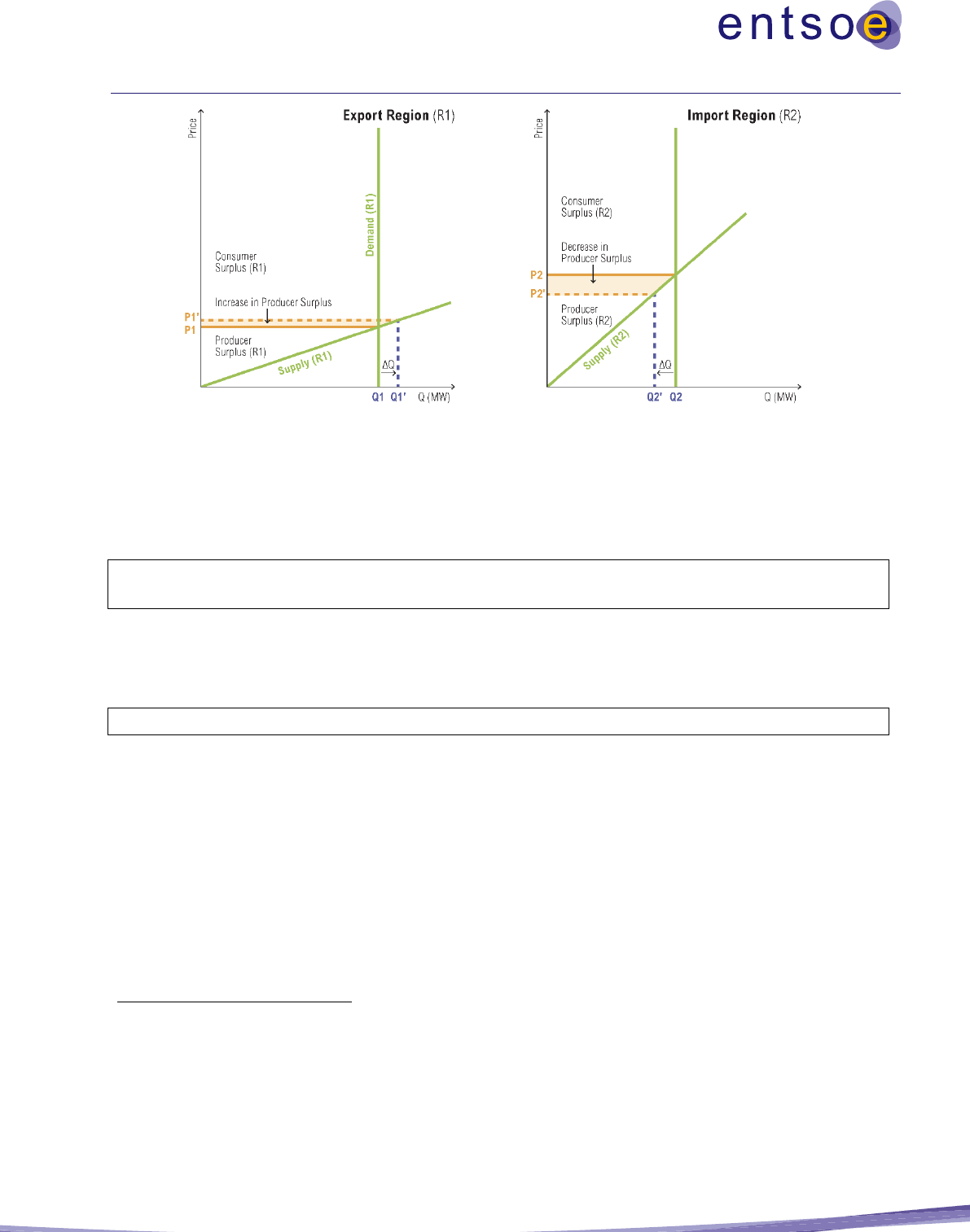
123
Figure 18: Change in producer surplus
The congestion rents with the project can be calculated from the price difference between the importing
and the exporting areas, multiplied by the additional power traded by the new link
58
.
The change in total congestion rent for a specific sector can be calculated as follows:
Change in total congestion rent = change of congestion rents on all links between import and export
areas
The cross-sector rent with the project can be calculated from the price difference between the coupled
sectors, the energy conversion efficiency and the additional power required for the energy conversion from
energy carrier A into B. The change in total cross-sector rent
59
for a specific sector is
Change in total cross sector rent = change of cross-sector rents between associated sectors
58
In a practical manner, it is calculated as the absolute value of (Marginal cost of Export Area – Marginal cost of Import Area) x flows on the
interconnector.
59
Further details on the calculation of cross-sector rents can be found in T. Felling and P. Fortenbacher, ‘Extended Social Welfare
Decomposition for Multi-Energy Systems,’ 2022 18th International Conference on the European Energy Market (EEM), 2022, pp. 1-7, doi:
10.1109/EEM54602.2022.9921010.
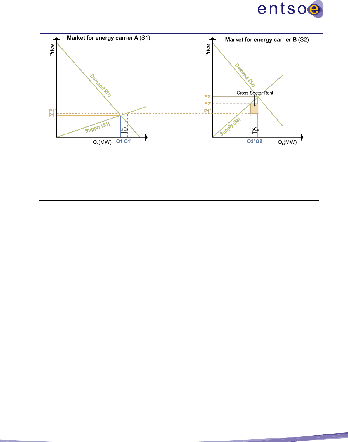
124
Figure 19: Illustration of sectorial market coupling. The cross-sector rent captures the benefit of sector coupling and describes
the welfare movement from sector A to B. It can be regarded as an additional welfare component.
The global benefit for each case is calculated by:
Benefit (for each time step) = sum of Total surpluses with the project (sum over all time steps) over
all sectors – sum of Total surpluses without the project (sum over all time steps) over all sectors
The total benefit for the horizon is calculated by summarising the benefit for all the hours of the year, which
is achieved through market studies.

125
III. Example of ΔNTC calculation
An example is provided below to illustrate how to calculate the ΔNTC. The example uses the TOOT
approach for one time step. The PINT approach is similar; only the position of the project towards the
reference network model changes.
The example is designed for a ΔNTC calculation across any boundary between bidding zones.
60
This
methodology should be performed over all the time steps of the year to calculate an annual ΔNTC to be
used for simulations.
Consider the example system as presented below. The following steps must be followed:
• Step 1: Perform load flow analysis on the reference network model in line with the security criteria
that consider the N-1 criterion.
• Step 2: Identify the total generation in zone X and Y (in the simple example, zone Z does not have
any generation or demand), which corresponds with at least one line loaded at exactly 100% under
N-1 condition (100% situation) in one of the areas around the border under consideration (i.e. X
and Y in the example), and with no other congestion, under the assumption that there are no
congestions in zone Z. The 100% situation can be created by performing a generation power-shift
61
in zones X and Y (and vice versa).
62
• Step 3: Repeat steps 1 and 2 on the reference network model from which the project has been
removed (TOOT of the project for which the ∆NTC shall be determined). This will provide the
values for generation in X and Y in the situation when one of the lines is loaded at exactly 100%
under N-1 without the project.
• Step 4: Calculate the ΔNTC as the difference between the generation situations that correspond
with the 100%-situations: ∆NTC equals the power shift.
• Step 5: Apply this process to both directions of power-flow across the boundary under analysis.
60
In principle, the method can also be applied to any type of boundary.
61
Which generators to use for the generation power-shift is highly context-dependent. As many different methods for the generation power-shift
can be applied without the possibility of identifying a preferable one, no favoured methodology for the generation power-shift is given in this
Guideline. But it should be mentioned that the generation power-shift can have a significant impact on the results and should, therefore, be chosen
carefully and with a detailed justification. In the likely case where the initial highest N-1 load may be higher or lower that 100%, a power shift
relative to the initial dispatch across the boundary is to be applied in order to reach 100% and find the corresponding power value. Depending on
the initial conditions, this power-shift would increase or reduce the reference power-flow.
62
If not possible, a load power-shift could also be performed
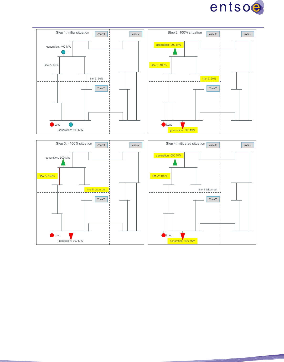
126
Figure 20: Qualitative example to illustrate the single steps, as described in the example above. It should be noted that the real
physical flow will also have a component across the boundary between zones X–Z and Z–Y.
The results of the calculations described in the steps above are illustrated in Table 12 below.
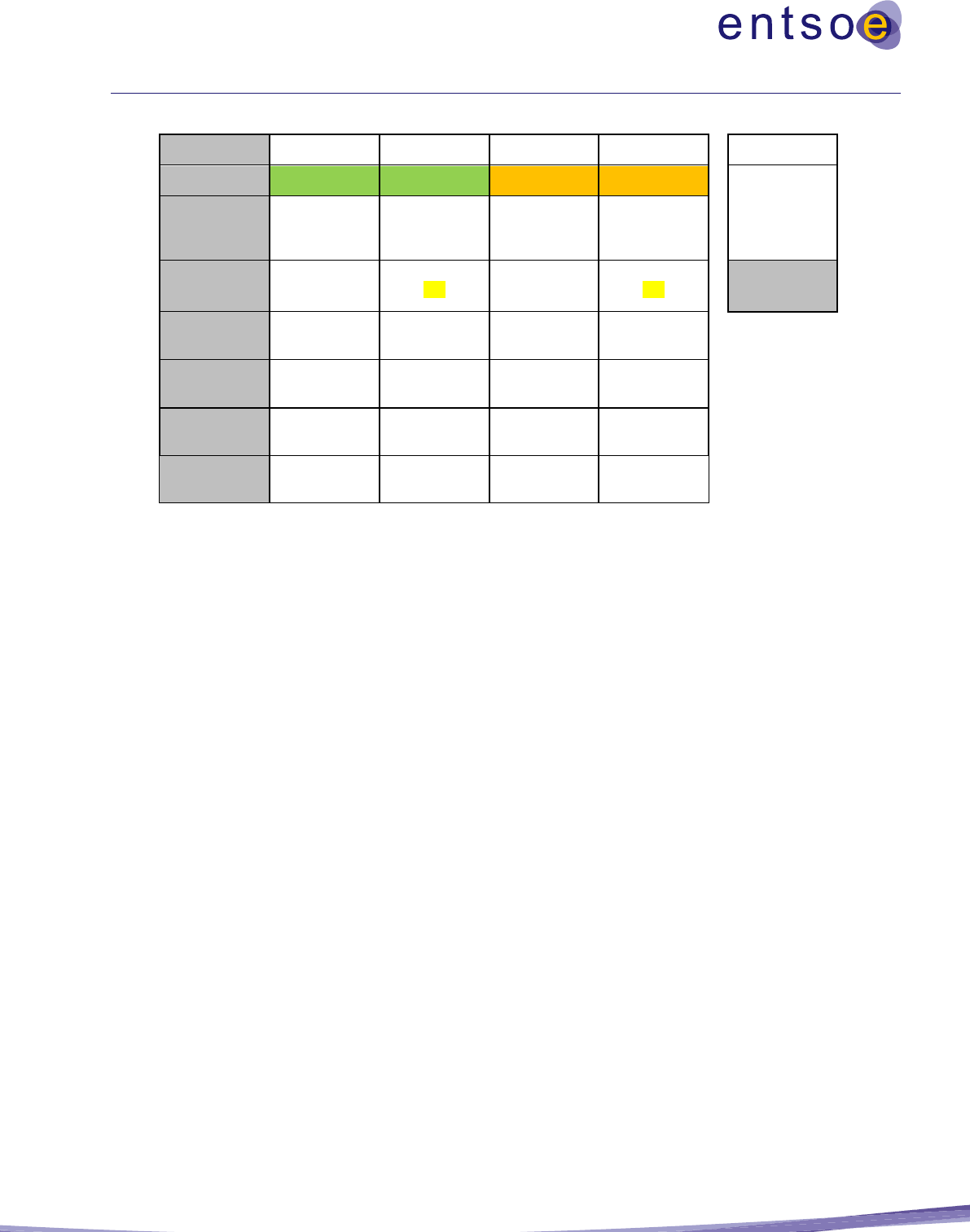
127
Table 20: Simplified example of ∆NTC increase from direction X to Y across a boundary.
Step 1
Step 2
Step 3
Step 4
Step 5
Incident
Line B in
Line B in
TOOT line B
TOOT line B
∆ NTC X > Y
[MW]
Situation
initial situation
100% situation
>100% situation
mitigated
situation, thus
back to 100%
Generation in
zone X
400
900
900
600
300
Generation in
zone Y
800
300
300
600
demand to be
covered
1200
1200
1200
1200
Line loading at
line A
80%
100%
150%
100%
Line loading at
line B
50%
80%
-
-
From the table above, it can be seen that:
• Step 1 denotes the initial situation where all projects are put in (including line B). No overloads
show up, illustrated by the line loadings in %.
• In Step 2, the generation power-shift has been done until one line is loaded at exact 100% (line A
in this example) under N-1 conditions. The power-shift-volume needed was 500 MW.
• In Step 3, line B is taken out as per the TOOT approach. The dispatch is fixed as it was after Step
2, with +500 MW in zone X and -500 MW in zone Y. The loading of line A became 150% (N-1).
• In Step 4, the generation power-shift is done in the opposite direction to that done in Step 2. This
reduces the load one line A to 100% (N-1). The remaining power-shift, compared to the initial
situation, is 200 MW. Hence, the project enables a power-shift increase of difference between initial
dispatch and final dispatch; thus, 500 MW – 200 MW = 300 MW.
• Step 5 illustrates the corresponding ∆NTC in the direction of X > Y across the boundary.
